Theory of Chromatic Vision Simulator 4.0
1. Overview
This paper describes the color transformation by which the app "Chromatic Vision Simulator" 4.0 simulates the appearance of an image for each type of color vision (protanope, deuteranope, tritanope). The essential point is that the color of each pixel of the image is mapped into the LMS space, which represents the responses of the cones, projected by the method of Brettel et al. [1] onto the surface that corresponds to the color appearance of a dichromat, and mapped back to the original color space. The framework of this paper is a reorganization, for version 4.0, of the mathematical expressions in the appendix of the README of the Android version 3.3.1 of the same app [2]. In addition, §7 states in outline the theory of displaying the name of the color that has been read.
1-1. Assumptions
The following are assumed throughout this paper.
- 1. White point: D65, (the defined value in the sRGB and Display P3 standards [3][4][5]). It is common to all conversions.
- 2. Observer: the XYZ of the colors of the image is that of the CIE 1931 2° standard observer [6] (the definition of XYZ [7][8]). Only the construction of the cone matrix (§4-1) and the chromaticity coordinates of the anchor stimuli of dichromacy (§5-1) use the color-matching functions of the CIE 1964 10° supplementary standard observer (the X10Y10Z10 system) [7] and their chromaticity coordinates, taken from Table 2 of JIS Z 8701 [9].
- 3. Color spaces: the input and the display are each either sRGB [3] or Display P3 [4][5]. The two share the same transfer function and differ only in the primaries (§2, §3).
- 4. Quantization: 8 bits ( to ). The encoded value is treated as a real number in obtained by dividing the pixel value by .
- 5. Chromatic adaptation: since the white points of the input and the display are both D65, no chromatic adaptation transform is applied.
- 6. Cone space: the conversion from XYZ to LMS uses a 3×3 matrix that keeps the shape of the Hunt–Pointer–Estévez (HPE) cones and is built from the 10° XYZ, normalized to D65 [9][10][11].
- 7. Types of color vision: complete dichromacy is simulated (protanopia is the absence of the L cone, deuteranopia of the M cone, and tritanopia of the S cone). The simulation strength is a value for showing the intermediate image between the color appearance of the most severe form of dichromacy of each type (100%) and the original image (0%). It does not simulate the color appearance of anomalous trichromacy (mild color vision deficiency) (§5).
- 8. Difference mode: the color difference is the Oklab distance between the original image and the simulated image, and the target is the simulation result including the strength (§8).
1-2. Notation
- : the components of linear RGB, taken in with white equal to . : the components of XYZ ( is for white).
- : the encoded RGB (each component , ). : the linear value (). The chromaticity coordinates use the same letter as the linear value , but in §3 and §4 they denote chromaticity coordinates.
- : the components of the cone responses (LMS). We write . For the D65 white, .
- : the XYZ → LMS conversion matrix. : the RGB → XYZ conversion matrix. : the matrix representing the projection onto a half-plane of a dichromat.
- : the strength parameter (). is complete dichromacy and is the original color.
1-3. Flow of the processing
For each pixel of the image, the processing is applied in the following order.
encoded RGB ──(§2) decoding──▶ linear RGB ──(§3, §4) matrices──▶ LMS
LMS ──(§5) projection onto a half-plane and mixing by strength──▶ LMS′
LMS′ ──(§4, §3) matrices──▶ linear RGB′ ──(§5-4) gamut limit──▶ ──(§2) encoding──▶ encoded RGB′
Difference mode (§8) displays the Oklab distance between LMS′ and the original LMS as brightness.
2. Transfer functions (gamma)
The relation between the encoded value (; for 8 bits, ) and the linear value () is defined as the transfer function [12]. The sRGB function of IEC 61966-2-1 [3] is used.
Decoding (encoded value to linear value):
Encoding (linear value to encoded value):
The two expressions are continuous at (), since . The transfer function of Display P3 is identical to that of sRGB.
Before encoding, values that have become negative outside the color gamut are replaced by (because a power of a negative number is undefined). Both the decoded and the encoded results are confined to the range to .
3. Conversion between RGB and XYZ
Let the linear RGB be the column vector , with the white point D65. The conversion matrices are derived from the chromaticities of the primaries and the white point as follows [8][12].
3-1. Derivation from the primaries and the white point
Let be the chromaticity of primary (), and define its direction vector
Let be the matrix having these vectors as columns, and let be the vector of the same form for the chromaticity of the white point. The condition that white () is mapped to , namely , determines the strength coefficients of the primaries, . The RGB → XYZ matrix is then
with which white has . The XYZ → RGB matrix is the exact inverse of .
3-2. sRGB
The chromaticities of the primaries are R, G, B, and the white point is D65 with (IEC 61966-2-1 [3]). By §3-1, the values derived in double precision are, to seven digits,
The forward matrix given by the standard to four decimal places coincides with these derived values rounded to four digits. The inverse matrix of the standard to four digits is the rounded inverse of the rounded four-digit forward matrix, and therefore differs from the inverse of the derived matrix above in the fourth digit.
3-3. Display P3
The chromaticities of the primaries are R, G, B, and the white point is D65 with (SMPTE EG 432-1 [4]; Apple's definition [5]). By §3-1 one obtains likewise
3-4. Exchanging color spaces
XYZ does not depend on the color space. Therefore, even when the input is sRGB and the display is Display P3, the computation after the conversion to LMS (§4) is common, and only the matrices of the input and the display need to be exchanged.
4. Conversion from XYZ to LMS
4-1. The cone matrix (the 10° version that keeps the shape of HPE)
The cone responses are given as a linear transformation of XYZ. This paper uses a 3×3 matrix that keeps the shape of the spectral sensitivities of the cones of Hunt–Pointer–Estévez (HPE) [10] and is built from the XYZ of the CIE 1964 10° supplementary standard observer (the X10Y10Z10 system; Table 2 of JIS Z 8701 [9]). The HPE transform from the CIE 1931 XYZ to the cone responses is expressed by the following matrix, normalized to the equal-energy white (see [11] for an exposition).
The matrix of the 10° version is found by unweighted least squares over all wavelengths (81 points at 5 nm intervals from 380 nm to 780 nm) so that the 10° color-matching functions (CIE 1964 [7]; the values are taken at every 5 nm from the 1 nm table of [13]) best reproduce the HPE cone sensitivities , where are the CIE 1931 2° color-matching functions (values also from [13]). Then each row is divided by the corresponding component of , so that the XYZ of the D65 white point (, §3-1) gives .
The derived values are, to five digits,
The 10° and 2° color-matching functions are not related exactly by a linear transformation, so the fit leaves a residual (at most 0.23; the maximum of the HPE sensitivities is about 1, and the residual is largest on the short-wavelength side near the S cone). This matrix is not a published standard but an approximation made for this paper, and the shape of the cones remains that of HPE (physical differences of the 10° cones, such as the effect of the macular pigment, are not reflected). The XYZ of the input colors (sRGB and Display P3) remains that of the 2° observer.
By this normalization the D65 white is mapped to . In the following, the straight line through this point is called the neutral axis.
4-2. Conversion between linear RGB and LMS
The conversion from linear RGB to LMS is given by the product of of Eq. (4) and of Eq. (11).
When the input and the display are sRGB, the values to seven digits are
When the input and the display are Display P3, they are
5. Simulation of dichromacy
5-1. Approximation by half-planes
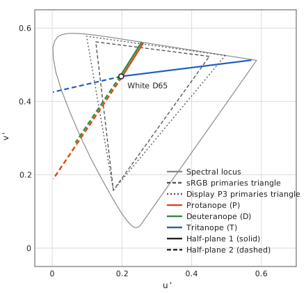
A dichromat lacks one of the three classes of cones. Two stimuli that differ only in the response of the missing cone cannot be distinguished, and in the LMS space the points on a straight line parallel to the axis of the missing component (a confusion line) look like the same color. Therefore the color appearance of a dichromat can be represented by points on a two-dimensional surface of the LMS space. Brettel et al. approximated this surface by two half-planes through the neutral axis and two anchor stimuli on the spectral locus (475 nm and 575 nm for protanopes and deuteranopes, and 485 nm and 660 nm for tritanopes) [1]. The two half-planes meet along the neutral axis.
Each half-plane passes through the origin and contains the LMS of the white and the LMS of an anchor stimulus. Writing the missing component as and the other two components as , a half-plane can be written in the form , and the condition of passing through and gives the coefficients
In this paper the chromaticity coordinates of the anchor stimuli are the spectral chromaticity coordinates of the CIE 1964 10° supplementary standard observer (the X10Y10Z10 system), taken from Table 2 of JIS Z 8701 [9] (five digits). The anchor stimuli and the cone matrix of §4-1 are both matched to the 10° observer; the chromaticity coordinates are used as the values and converted to LMS by the matrix of §4-1. The XYZ of the colors of the image remains that of the 2° observer (the definition of sRGB) (since a plane passes through the origin, the magnitude of an anchor stimulus does not affect the coefficients).
| Wavelength | |||
|---|---|---|---|
| 475 nm | 0.09573 | 0.15909 | 0.74518 |
| 485 nm | 0.04519 | 0.32754 | 0.62727 |
| 575 nm | 0.50964 | 0.49036 | 0.00000 |
| 660 nm | 0.71679 | 0.28321 | 0.00000 |
The correspondence between the two half-planes and the anchor stimuli is as follows: for protanopes and deuteranopes, the side where the response of is small (, ) corresponds to 575 nm and the other side to 475 nm; for tritanopes, the side corresponds to 660 nm and the other side to 485 nm (the boundary of the selection is given in §5-2). The white is the LMS of the D65 white (the normalization of §4-1). The simulated color is the point obtained from the original color by replacing only the missing component, and can be written with a matrix (a projection parallel to the missing axis). Since , Eq. (17) gives exactly, and the half-plane contains the neutral axis. The coefficients are, to five digits, as follows.
Protanopia (absence of the L cone; ):
Deuteranopia (absence of the M cone; ):
Tritanopia (absence of the S cone; ):
The coefficients of this paper (from the 10° anchors and the 10° version of the cone matrix) are compared below with the values of version 2.x of the original app (HPE 2° cones with 10° anchors; computed from the four-digit XYZ of the anchors and the white of the four-digit sRGB matrix). Because the cone matrix differs, the difference is at most (the coefficient of half-plane 2 for the tritanope).
| Type | Half-plane | This paper | Original 2.x |
|---|---|---|---|
| Protanope | 1 | ||
| Protanope | 2 | ||
| Deuteranope | 1 | ||
| Deuteranope | 2 | ||
| Tritanope | 1 | ||
| Tritanope | 2 |
5-2. Selection of the half-plane
Which of the two half-planes is used is determined by which side of the neutral axis the original color lies on. The boundary of the selection is the plane containing the neutral axis and the axis of the missing cone ( axis for protanopes, axis for deuteranopes, axis for tritanopes): for protanopes, for deuteranopes, and for tritanopes. At a point on this boundary the two half-planes give the same replacement because . For protanopes, for example, at ,
Therefore the result of the simulation is continuous at the boundary.
5-3. Mixing by strength
The simulation with strength () is given by an interpolation between the original color and the complete dichromatic simulation . Version 2.x of the original app interpolated and linearly in the LMS space. In this paper (version 4.0), both are first limited to the gamut of the display, and then interpolated linearly in the Oklab space [14].
(1) Limiting to the gamut. The linear RGB of the display is given by ( of Eq. (30)); it is limited componentwise to the range to and converted back to LMS.
(2) Conversion to Oklab. The LMS is converted back to XYZ and mapped by Ottosson's matrix to the cone-like responses of Oklab; the cube root of each component is taken, and the matrix gives .
The cube root is the componentwise signed cube root (). The matrices are as follows ( maps XYZ (D65, with for white) to , and maps the cube roots of to ).
(3) Inverse conversion. From back to LMS, apply , then the componentwise cube, then , then .
where is the componentwise cube. The values of the inverse matrices are as follows.
(4) Interpolation. The Oklab values of the limited and are interpolated linearly with the strength and converted back to LMS.
where is the inverse conversion of Eq. (25). At the original color inside the gamut is unchanged (), and at the result is .
The reason for limiting before the interpolation: for vivid blues and purples, the result of the dichromat simulation has negative components in linear RGB (outside the gamut). If the interpolation in Oklab is performed without limiting, the intermediate colors of the interpolation move outside the gamut, the components stick to in the final limiting, and the color jumps abruptly as the strength is raised. If both end points are limited to the gamut before the interpolation, the intermediate colors also stay inside the gamut.
Compared with the linear interpolation in LMS, the interpolation in Oklab makes the change of appearance closer to uniform when the strength is moved in equal steps. When the strength was moved in steps of , the maximum divided by the minimum of the Oklab distances between adjacent steps was, in a test with six representative colors and three types, at most for the linear interpolation in LMS and at most for the interpolation in Oklab.
A method for displaying the difference in color of the simulation result on the screen is described in §8.
5-4. Limiting to the gamut
Since both end points were limited to the gamut before the mixing (Eq. (22)), the mixed color lies inside the gamut except for numerical errors. The limiting after the conversion back to linear RGB is a safeguard against these errors. Components that have become negative outside the gamut are limited to , and components exceeding are limited to .
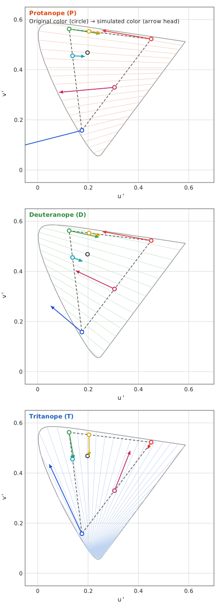
When the simulation with is applied to all the colors of sRGB (the points obtained by taking 33 equally spaced steps of the encoded value for each component), the proportions of the colors that fall outside the gamut before the limiting () are as follows. Achromatic colors (colors on the neutral axis) do not move.
| Type | Colors with a negative component | Colors with a component exceeding |
|---|---|---|
| Protanope | 29.1% | 10.6% |
| Deuteranope | 23.2% | 4.3% |
| Tritanope | 8.2% | 1.9% |
6. The overall transformation
Including the case where the color spaces of the input and the display differ, the transformation from the encoded input to the encoded output is written as the composition of §2 to §5.
Here is the encoding of Eq. (2) (component by component), is the limit of Eq. (28), and is the mixture of Eq. (27). The used in the mixture is ( is the decoding of Eq. (1)), , and is the matrix selected from Eqs. (18) to (20) according to the type and the position of . With the matrix of the color space of the input and that of the display (both of the form of Eq. (4)),
The numerical values for the case where the input and the display are both sRGB or both Display P3 are given in §4-2.
7. Display of color names
This section states, in outline only, the theory of the process that reads the color at one point of an image and displays its color name and color values (the display of color names). The names are the systematic color names and the traditional color names of the Japanese Industrial Standard JIS Z 8102 [15] (the default of the Japanese screen). The English color names are described in §7-6. Below, the XYZ of a color is the D65 value obtained in §3, and the reading is made on the original image (before the simulation).
7-1. How the color to read is determined
A single pixel is easily affected by sensor noise and fine patterns. The color to read is therefore the Gaussian-weighted average, in the Oklab space [14], of the pixels around the pointed position. From the XYZ (D65) of pixel , the Oklab value () is computed with the same matrices as in Eq. (23), and the weight at the position (the distance of the pixel from the pointed position, in pixels) is
The sum is taken over the pixels within of the pointed position in both directions, and converted back to XYZ by the inverse Oklab transformation is the color to read. is fixed as a length on the screen (6 pt) and converted to the size of the pixels of the original image, so that the same area on the screen is read regardless of zooming. Oklab is highly uniform perceptually and has small hue shifts, so the average is a color that looks intermediate.
7-2. Systematic color names
A systematic color name is determined by expressing the color in Munsell hue , value and chroma and applying it to the regions defined by JIS Z 8102. The values of the Munsell system follow JIS Z 8721 [16] and ASTM D1535 [17].
Value. The relation between the luminance factor (white is ) and the Munsell value is the fifth-degree polynomial
[16] (the coefficients are the values of JIS Z 8721; those given for [17] differ in the last digit, see the note to reference [17]). This function increases monotonically for , so is obtained by solving the exact inverse of Eq. (32) numerically.
Hue and chroma. The Munsell renotation table [17][18] gives the chromaticities of the grid points of hue and chroma for each value level. The XYZ of the color to read is converted to the chromaticity adapted to illuminant C (§7-4); for each value level, the position of the chromaticity point inside the cell of the grid that contains it is found by inverse bilinear interpolation, which gives hue and chroma. The results of the two levels that enclose the point are interpolated linearly in value. A color whose chroma is less than is achromatic (). When the chromaticity point lies outside the table, the chromaticity is shrunk toward the white point of illuminant C while the value and the hue are kept, and the outermost point that falls inside the table is used.
Regions of systematic color names. JIS Z 8102 defines the systematic color names as a table of rectangles in Munsell hue, value and chroma. The rounded to five digits is applied to the rectangles of this table (boundaries included) to find the symbol of the systematic color, and the symbol is turned into a name (for example, light grayish greenish yellow) [15].
7-3. Traditional color names
Of the traditional color names of JIS Z 8102, the 267 that are defined by Munsell values each use their Munsell value [15]. From the Munsell value of each traditional color, the XYZ under illuminant C is obtained and converted to D65 by the chromatic adaptation of §7-4, which gives the CIELAB value (D65 white, ; formulas in [7]). The traditional color nearest to the CIELAB value of the color to read is selected as follows.
The distance is CIEDE2000 (CIE 142:2001 [19]; computed with the formulas of [20]) by default. When the distance to the nearest color exceeds , that traditional color cannot be called close, and a "?" is appended to the name. A traditional color whose coordinates are shared by several names is shown with all of them.
7-4. Chromatic adaptation and the observer
The Munsell values and the traditional colors of JIS Z 8102 are defined under illuminant C and the CIE 1931 2° standard observer, whereas the white of the screen is D65. Therefore the XYZ of D65 is adapted to illuminant C before it is converted to Munsell values, and the XYZ of the traditional colors is adapted to D65 before it is converted to CIELAB. The adaptation is a linear transformation of the Von Kries type in the cone space of Hunt–Pointer–Estévez [10][11]. Let (chromaticity ) and (chromaticity ) be the XYZ of the white points (); with the matrix of Eq. (9) (the HPE for 2°), the transformation from D65 to C is
(the fraction is the componentwise ratio). The transformation from C to D65 is its inverse. The used here is that of the 2° observer and is distinct from of the simulation in §4 (the matrix matched to 10°). As in §1-1, the XYZ of the colors of the image is that of the 2° observer.
7-5. Available formats
The color to read (XYZ of D65) can be displayed in the following formats.
- Munsell value (§7-2; written in the form "5GY 7/8") and the systematic and traditional color names (§7-2, §7-3).
- sRGB: the encoded 8-bit values (§2, §3-2). Values outside the gamut are limited to –.
- XYZ (D65, is for white) and xyY (the chromaticity coordinates and ), defined as in [7].
- CIELAB and CIELUV (D65 white; defined as in [7]).
- Oklab (the same transformation as Eq. (23) [14]).
8. Computing the color difference (difference mode)
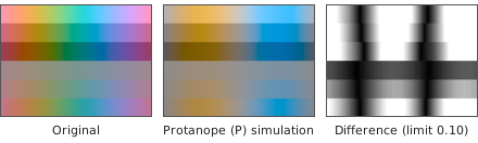
Difference mode displays, for each pixel of the image, the difference between the original color and the simulated color as brightness. The larger the difference, the brighter the pixel; a pixel with no difference is black. This section describes how the difference is computed.
8-1. Distance
Let be the LMS of the original color and the result of the simulation at strength (Eq. (27)). The distance is the Euclidean distance in Oklab space [14]. The conversion to Oklab is the same as the one used for the strength blend (Eqs. (22)–(24)): the original color is clipped to the display gamut by Eq. (22) and then converted to Oklab, and the simulated color uses the Oklab value obtained in the blend.
Here is the Euclidean distance over the three components . By Eq. (27), , so the distance is proportional to the strength.
An implementation therefore only needs to convert the result of the full dichromat simulation () to Oklab, take the distance, and multiply by . Lowering the strength darkens the whole difference image. Because the gamut clip is applied before the distance is taken, for colors the display cannot show (vivid blues and purples) only the part of the difference that is visible on the display is counted.
8-2. Mapping to brightness
The distance is divided by an upper limit to give the brightness ().
is black (no difference); is white (a difference at or above the limit); in between the mapping is linear. The three output components are itself, used directly as an encoded value (the value after the encoding of Eq. (2)).
The user adjusts with the strength slider (in difference mode the slider represents the upper limit, not the strength). The slider value () maps linearly to the limit.
ranges from to , and the default is at . A smaller makes even small differences close to white; a larger makes only large differences close to white.
Pixel values are 8-bit, so brightness is displayed in steps of . At , differences smaller than about become black. Small differences caused by sensor noise also appear when is small.
Figure 3 shows an example of the difference image.
8-3. Why Oklab
The same space. The color difference is computed in the same Oklab space as the strength blend (§5-3) and the averaging of the read color (§7-1). The conversion matrices (Eq. (24)) and the implementation are shared, so the simulated result and the difference are consistent on one scale.
A simple distance. Oklab has high perceptual uniformity [14], so the Euclidean distance is already close to the perceived difference. CIEDE2000 [19][20] weights hue, chroma, and lightness with a complicated formula (trigonometric functions and case distinctions) that is not suited to per-pixel (shader) processing.
Relation to CIEDE2000. The differences between before and after a simulation are larger than the small color differences that CIEDE2000 was designed for. We measured the correspondence on pixels of a 128-color chart, hue bands, the 267 JIS common colors, Ishihara-like dots, and five photographs (types 1, 2, and 3, strength 1). The table gives the median of pixels whose Oklab distance is near each value (±10%), and the median Oklab distance of pixels whose is near each value.
| Oklab distance | (median, quartiles) | Oklab distance (median, quartiles) | |
|---|---|---|---|
| 0.05 | 14 (13–16) | 5 | 0.013 (0.011–0.018) |
| 0.10 | 22 (20–24) | 10 | 0.028 (0.025–0.035) |
| 0.20 | 32 (29–34) | 20 | 0.082 (0.069–0.097) |
| — | — | 40 | 0.238 (0.203–0.260) |
The default limit corresponds to : a difference that anyone can see when the two colors are placed side by side. To turn differences of white, set the limit to about . The correspondence varies with color, and the values above are guides based on the pixel statistics described. In its gamut mapping, the W3C's CSS Color Module Level 4 takes one JND (just noticeable difference) in the OkLCh color space to be , measured by , the Euclidean distance over the Oklab components (§20.3 of the same document) [21]. The distance in this section (Eq. (35)) is on the same scale as . The lower end of the limit, , is half of that.
8-4. Limitations
- The Euclidean distance in Oklab approximates perceived difference. For large differences the correspondence between distance and appearance varies with color (as does the correspondence in the table). For measuring color differences on a strict scale, use or a similar formula.
- The quantity is the difference between the original and the simulation. It does not measure how easily two colors within the image can be told apart. The simulation is a full dichromat (strength ) or an interpolation by strength; it is not the appearance of anomalous trichromacy itself (§5).
- It depends on the display gamut. The distance is measured on colors clipped to the display gamut (Eq. (22)). On a Display P3 screen the clip differs from sRGB, so values change, especially for vivid colors.
- The displayed brightness has 8-bit steps. Small differences and noise may appear or turn black depending on the limit (§8-2).
- The difference saturates at the limit. All differences with are shown as white, so differences in their magnitude cannot be seen.
7-6. Sources of the English color names
Systematic color names (ISCC-NBS). They follow the ISCC-NBS method of designating colors [22]. The space of Munsell hue, value, and chroma is divided into 267 regions (color-name blocks), and each region is given an English systematic color name. The boundaries of the regions are taken from the figures of NBS SP 440 [23].
Traditional color names (TCCA). They follow NBS Research Paper RP1700 [25], which measured 238 colors, the 216 colors of the standard color card of the Textile Color Card Association (TCCA) and the 22 colors of the U.S. Army color card, by spectrophotometry and other methods and gave each card a Munsell renotation. The application uses 178 names: 156 names of TCCA cards, 9 names of Army cards, and the 13 basic terms. The nearest-neighbor search is the same as for the JIS traditional color names (§7-3). The 13 basic terms (such as red and pink) use the colors of ISCC-NBS Level 1 [22], and their colors are the Munsell values of the block centers in Kelly's report [24]. The TCCA and Army cards of the same names are not used.
References
[1] H. Brettel, F. Viénot, and J. D. Mollon, "Computerized simulation of color appearance for dichromats", Journal of the Optical Society of America A, vol. 14, no. 10, pp. 2647–2655, 1997. doi:10.1364/JOSAA.14.002647
[2] K. Asada, "Chromatic Vision Simulator", README of the Android source code (code version 3.3.1; the README itself is headed "Android version 3.0") (appendix: mathematical expressions for color vision simulation), GitHub repository asada0/ChromaticVisionSimulator, 2018, MIT License. https://github.com/asada0/ChromaticVisionSimulator (accessed 25 October 2026)
[3] IEC 61966-2-1:1999, Multimedia systems and equipment — Colour measurement and management — Part 2-1: Colour management — Default RGB colour space — sRGB, International Electrotechnical Commission; and Amendment 1:2003 (published 23 January 2003).
[4] SMPTE EG 432-1:2010, Digital Source Processing — Color Processing for D-Cinema, Society of Motion Picture and Television Engineers, 10 November 2010. doi:10.5594/SMPTE.EG432-1.2010
[5] Apple Inc., "Display P3", Three Component Color Encoding Registry (ICC Registry), International Color Consortium, version 1.0, 9 February 2022. https://registry.color.org/rgb-registry/displayp3 (accessed 22 October 2026). See also Apple Developer Documentation, CGColorSpace.displayP3, https://developer.apple.com/documentation/coregraphics/cgcolorspace/displayp3 (accessed 22 October 2026).
[6] T. Smith and J. Guild, "The C.I.E. colorimetric standards and their use", Transactions of the Optical Society, vol. 33, no. 3, pp. 73–134, 1931–32. doi:10.1088/1475-4878/33/3/301
[7] CIE 15:2004, Colorimetry, 3rd ed., Commission Internationale de l'Éclairage, 2004, ISBN 978-3-901906-33-6 (since superseded by CIE 015:2018).
[8] G. Wyszecki and W. S. Stiles, Color Science: Concepts and Methods, Quantitative Data and Formulae, 2nd ed., John Wiley & Sons, 1982, ISBN 978-0-471-02106-3.
[9] JIS Z 8701:1999, Colour specification — The CIE 1931 standard colorimetric system and the CIE 1964 supplementary standard colorimetric system (in Japanese: 色の表示方法 — XYZ 表色系及び X10Y10Z10 表色系), Japanese Standards Association, 1999. Table 2 (spectral chromaticity coordinates of the X10Y10Z10 system). Note: a secondary source states that this standard was withdrawn when JIS Z 8781-3 was established in 2016 (not confirmed against the JISC original). The values of Table 2 used here were checked against the JIS Handbook 61 (Color).
[10] R. W. G. Hunt and M. R. Pointer, "A colour-appearance transform for the CIE 1931 standard colorimetric observer", Color Research & Application, vol. 10, no. 3, pp. 165–179, 1985. doi:10.1002/col.5080100306
[11] M. D. Fairchild, Color Appearance Models, 3rd ed., John Wiley & Sons, 2013, ISBN 978-1-119-96703-3. doi:10.1002/9781118653128
[12] C. Poynton, Digital Video and HD: Algorithms and Interfaces, 2nd ed., Morgan Kaufmann, 2012, ISBN 978-0-12-391926-7.
[13] Colour & Vision Research Laboratory, UCL Institute of Ophthalmology, "CIE 1931 2-deg XYZ color matching functions (ciexyz31_1.csv, 1 nm steps)" and "CIE 1964 10-deg XYZ color matching functions (ciexyz64_1.csv, 1 nm steps)", database of the Colour & Vision Research Laboratory, http://cvrl.ioo.ucl.ac.uk/cmfs.htm (accessed 26 October 2026).
[14] B. Ottosson, "A perceptual color space for image processing", blog post, 23 December 2020, https://bottosson.github.io/posts/oklab/ (accessed 26 October 2026).
[15] JIS Z 8102:2001, 物体色の色名(Names of non-luminous object colours), 日本規格協会(Japanese Standards Association), 2001. Note: public sources give 269 traditional color names. This document uses the 267 of them that are defined by Munsell values (the content of the remaining names was not confirmed against the original standard).
[16] JIS Z 8721:1993, 色の表示方法-三属性による表示(Colour specification — Specification according to their three attributes), 日本規格協会(Japanese Standards Association), 1993. Note: the coefficients of Eq. (32) are the values of this standard.
[17] ASTM D1535-14 (2023), Standard Practice for Specifying Color by the Munsell System, ASTM International, reapproved 2023. https://store.astm.org/d1535-14r23.html (accessed 26 October 2026) Note: Eq. (32) uses the coefficients of [16]. The coefficients of this standard given by a secondary source (1.1914, −0.22533, 0.23352, −0.020484, 0.00081939) differ in the last digit; the difference is at most 0.003 in Y (percent scale). The original texts of [16] and [17] were not read.
[18] S. M. Newhall, D. Nickerson, and D. B. Judd, "Final report of the O.S.A. subcommittee on the spacing of the Munsell colors", Journal of the Optical Society of America, vol. 33, no. 7, pp. 385–418, 1943. doi:10.1364/JOSA.33.000385
[19] CIE 142:2001, Improvement to industrial colour-difference evaluation, Commission Internationale de l'Éclairage, Vienna, 2001, ISBN 978-3-901906-08-4.
[20] G. Sharma, W. Wu, and E. N. Dalal, "The CIEDE2000 color-difference formula: Implementation notes, supplementary test data, and mathematical observations", Color Research & Application, vol. 30, no. 1, pp. 21–30, 2005. doi:10.1002/col.20070
[21] World Wide Web Consortium (W3C), "CSS Color Module Level 4", Candidate Recommendation Draft, 27 October 2026, §14.2.1 (Gamut Mapping: "For the OkLCh color space, one JND is an OkLCh difference of 0.02") and §20.3 (ΔEOK, defined as the Euclidean distance in Oklab color space). https://www.w3.org/TR/css-color-4/ (accessed 28 October 2026)
[22] K. L. Kelly and D. B. Judd, "The ISCC-NBS Method of Designating Colors and a Dictionary of Color Names", NBS Circular 553, National Bureau of Standards, 1955.
[23] K. L. Kelly and D. B. Judd, "Color: Universal Language and Dictionary of Names", NBS Special Publication 440, National Bureau of Standards, 1976. doi:10.6028/NBS.SP.440
[24] K. L. Kelly, "Central Notations for the Revised ISCC-NBS Color-Name Blocks", Journal of Research of the National Bureau of Standards, vol. 61, no. 5, pp. 427–431, 1958 (Research Paper 2911).
[25] G. Reimann, D. B. Judd, and H. J. Keegan, "Spectrophotometric and Colorimetric Determination of the Colors of the TCCA Standard Color Cards", Journal of Research of the National Bureau of Standards, vol. 36, no. 3, p. 209, 1946 (Research Paper RP1700).