Chromatic Glass

Theory of Iro no Megane (Chromatic Glass) 3.0

1. Overview

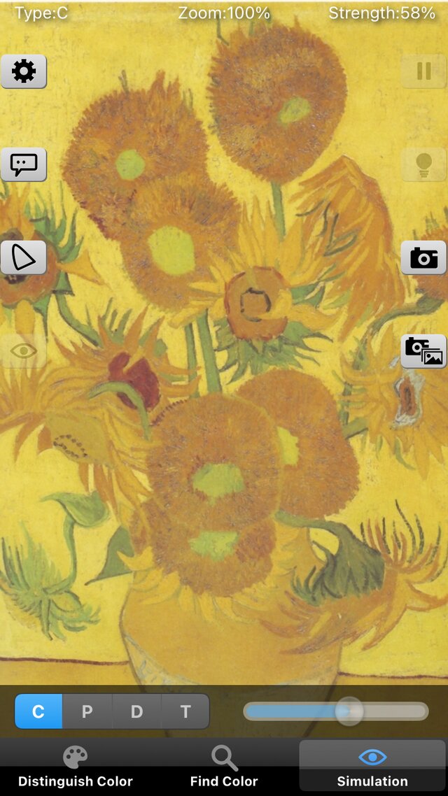
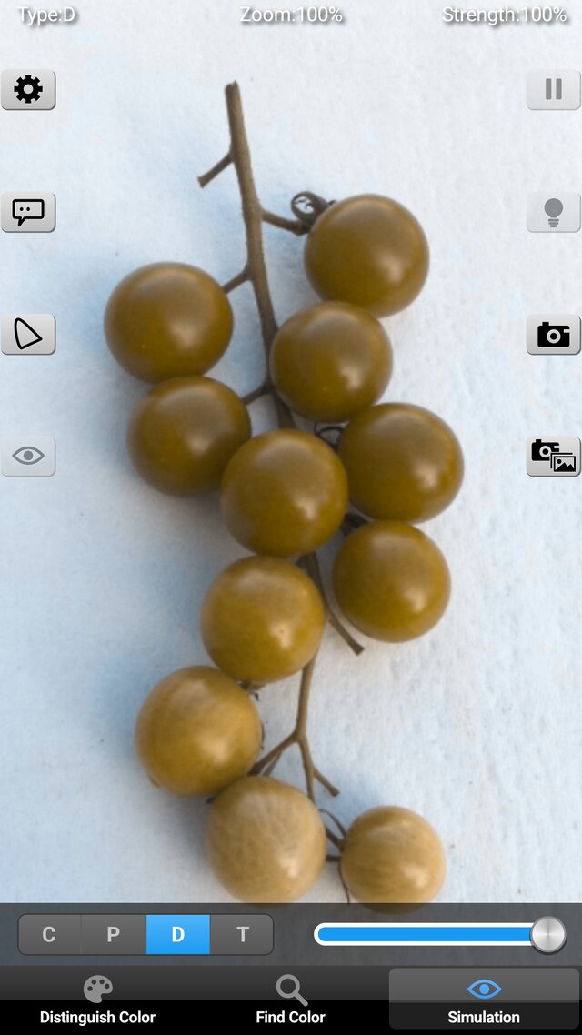
"Chromatic Glass" has three functions, switched with the tab bar at the bottom of the screen.

Distinguish and Find differ in which colors are changed, and share how they are changed (§7). Both focus on the difference in color that the person finds hard to distinguish. A person of type 1, 2 or 3 has a response of one of the L, M, S cones that differs from other people's, and finds it hard to distinguish two colors that differ only in that cone's response. The app moves colors in a direction different from that difference in cone response, so that colors that are hard to tell apart move to different colors.

In addition, there is a display of the name of the color under the cursor. It works as in Chromatic Vision Simulator 4.0 (§9).

As in the theory of Chromatic Vision Simulator 4.0, this paper gives all equations and constants down to the transfer function, the color space matrices, the cone matrix, the chromaticity diagram and the uniform color spaces, and then describes, with equations, how zones are decided (three methods), how colors are changed, and how Find colors works.

1-1. Assumptions

The following hold throughout this paper.

1. 1. White point: D65, $(x,y)=(0.3127,\,0.3290)$, $(u',v')=(0.19783,\,0.46832)$ (the defined values of sRGB and Display P3 [3][4][5]). It is common to all conversions.

1. 2. Observer: The XYZ of image colors is for the CIE 1931 2° standard observer [6] (definition of XYZ [7][8]). For the construction of the cone matrix (§4) and for the chromaticity coordinates of the anchor stimuli of the boost method (§7-5), the color matching functions of the CIE 1964 10° supplementary standard observer (X10Y10Z10 system) [7] and their chromaticity coordinates (JIS Z 8701, Appendix Table 2 [9]) are used.

1. 3. Color space: Input and display are each sRGB [3] or Display P3 [4][5]. They have the same transfer function and differ only in primaries (§2, §3). Numerical values and figures below are for sRGB unless noted.

1. 4. Quantization: 8 bits ($0$ to $255$). An encoded value is the pixel value divided by $255$, a real number from $0$ to $1$.

1. 5. Chromatic adaptation: Input and display both have the D65 white point, so no chromatic adaptation transform is applied.

1. 6. Cone space: XYZ is converted to LMS with the same matrix as Chromatic Vision Simulator 4.0 (a matrix that keeps the shape of the Hunt–Pointer–Estévez (HPE) cones, built to match the 10° XYZ and normalized to D65) [9][10][11].

1. 7. Color vision types: Types 1, 2 and 3 are the types for which the response of the L, M and S cone, respectively, differs from other people's. In calculation they are treated with a dichromat model that has no response from that cone, The simulation strength is a value for showing the intermediate image between the color appearance of the most severe form of dichromacy of each type (100%) and the original image (0%). It does not simulate the color appearance of anomalous trichromacy (mild color vision deficiency) (Simulation, §9).

1. 8. Display: A changed color is confined to $0$–$1$ of the linear RGB of the display color space and then encoded. When the color space differs between input and display (for example, Display P3 input and sRGB display), the calculations from §4 on are common; only the input and display matrices are replaced.

1-2. Notation

• $R,\,G,\,B$: components of linear RGB, from $0$ to $1$, white being $1$. $X,\,Y,\,Z$: components of XYZ ($Y$ is $1$ for white).
• $\mathbf{c}$: color of a pixel (XYZ). Encoded RGB (components $V$, $0\le V\le 1$) is written $\mathbf{c}_{\mathrm{in}}$, $\mathbf{c}_{\mathrm{out}}$.
• $L,\,M,\,S$: cone responses (LMS). $\mathbf{q}=(L,M,S)^{\mathsf T}$. For D65 white, $\mathbf{q}=(1,1,1)^{\mathsf T}$.
• $M$: matrix from linear RGB to XYZ. $M_{\mathrm{LMS}}$: matrix from XYZ to LMS.
• $u',v'$: CIE 1976 UCS chromaticity coordinates. $L^*,u^*,v^*$: CIELUV. $L,a,b$: Oklab (the same symbol as the cone response $L$, but used only in §5-3 and §6-5).
• $P$: zone position (red primary $0$, green primary $1$; for type 3, green $0$, blue $1$). The slider value is $s=1-P$.
• $f$: change magnitude ($0$ to $0.5$). $\mathrm{age}$: color rotation (one turn is $0$ to $1$). $w$: zone width, $a_Z$: zone start (slider value). $w_S$: width of the range in Find colors.

1-3. Processing flow

The following is applied to each pixel of the image, in this order.

encoded RGB ──(§2) decode──▶ linear RGB ──(§3, §4) matrices──▶ XYZ, LMS
   Distinguish:  decide pixels inside the zone by the zone position P (§6) ─┐
   Find:         decide pixels near the target by the u′v′ distance (§8)   ─┴▶ selected pixels
selected pixels ──(§7) change in CIELUV, confine to the gamut triangle──▶ changed XYZ
changed XYZ ──(§4) LMS──▶ (overlay of §9 Simulation, if on) ──▶ display linear RGB (clipped to 0–1) ──(§2) encode──▶ encoded RGB

2. Transfer function (gamma)

The relation between the encoded value $V$ ($0\le V\le 1$; for 8 bits, $\frac{\text{pixel value}}{255}$) and the linear value $x$ ($0\le x\le 1$) is defined as the transfer function [12]. The sRGB function of IEC 61966-2-1 [3] is used.

Decoding (from encoded to linear):

Encoding (from linear to encoded):

The two equations are continuous at $V=0.04045$ ($x=0.0031308$) ($\frac{0.04045}{12.92}=0.0031308$). The transfer function of Display P3 is identical to that of sRGB.

Before encoding, values that became negative outside the gamut are replaced by $0$ (a power of a negative number is undefined). The results of decoding and encoding are both clipped to $0$–$1$.

3. Conversion between RGB and XYZ

Linear RGB is the column vector $(R,G,B)^{\mathsf T}$, and the white point is D65. The conversion matrices are derived from the chromaticities of the primaries and the white point as follows [8][12].

3-1. Derivation from primaries and white point

Let the chromaticity of primary $i$ ($i=\mathrm{R},\mathrm{G},\mathrm{B}$) be $(x_i,y_i)$, and let its direction vector be

Let $P=[\mathbf{p}_{\mathrm R}\ \mathbf{p}_{\mathrm G}\ \mathbf{p}_{\mathrm B}]$ be the matrix with these as columns, and $\mathbf{W}$ the vector of the same form for the white point chromaticity $(x_w,y_w)$. From the condition $P\mathbf{S}=\mathbf{W}$ that white ($R=G=B=1$) maps to $\mathbf{W}$, the strength coefficients of the primaries are $\mathbf{S}=P^{-1}\mathbf{W}$. The RGB-to-XYZ matrix is then

and white has $Y=1$. The XYZ-to-RGB matrix is the exact inverse $M^{-1}$ of $M$.

3-2. sRGB

The chromaticities of the primaries are R$(0.64,\,0.33)$, G$(0.30,\,0.60)$, B$(0.15,\,0.06)$, and the white point is D65, $(x,y)=(0.3127,\,0.3290)$ (IEC 61966-2-1 [3]). By §3-1, the double-precision derived values to 7 digits are as follows.

3-3. Display P3

The chromaticities of the primaries are R$(0.680,\,0.320)$, G$(0.265,\,0.690)$, B$(0.150,\,0.060)$, and the white point is D65, $(0.3127,\,0.3290)$ (SMPTE EG 432-1 [4], Apple's definition [5]). By §3-1, likewise:

3-4. Replacing the color space

XYZ does not depend on the color space. Therefore, even if the input is sRGB and the display is Display P3, the calculations from the conversion to LMS (§4) on are common, and only the input and display matrices need be replaced. All constants of the calculation (chromaticities of the gamut primaries, constants of the zone) are computed from the primaries and white of the display color space.

4. Conversion from XYZ to LMS

4-1. Cone matrix (a 10° matrix keeping the shape of HPE)

The cone responses $\mathbf{q}=(L,M,S)^{\mathsf T}$ are given as a linear transform of XYZ. As in Chromatic Vision Simulator 4.0, this paper uses a 3×3 matrix that keeps the shape of the spectral sensitivities of the Hunt–Pointer–Estévez (HPE) cones [10], built from the XYZ of the CIE 1964 10° supplementary standard observer (X10Y10Z10; JIS Z 8701, Appendix Table 2 [9]). The HPE transform is expressed by the following matrix from CIE 1931 XYZ to cone responses (the form normalized to equal-energy white; see [11]).

The matrix $M_{\mathrm{raw}}$ for the 10° observer is found by unweighted least squares over all wavelengths $\lambda$ (81 points, 380 to 780 nm at 5 nm steps), so that the 10° color matching functions reproduce the HPE cone sensitivities as well as possible. The 10° color matching functions are $\bar{\mathbf{x}}^{(10)}(\lambda)=(\bar x^{(10)},\bar y^{(10)},\bar z^{(10)})^{\mathsf T}$ (CIE 1964 [7]), and the HPE cone sensitivities are $M_{\mathrm{E}}\,\bar{\mathbf{x}}^{(2)}(\lambda)$, where $\bar{\mathbf{x}}^{(2)}(\lambda)$ are the CIE 1931 2° color matching functions. Both sets of values are taken every 5 nm from the 1 nm tables of [13]. The rows are then normalized by dividing by the corresponding component of $M_{\mathrm{raw}}\mathbf{W}$, so that the XYZ of the D65 white point ($\mathbf{W}$, §3-1) gives $L=M=S=1$.

The values found are as follows, to 5 digits.

This matrix is not a published standard but an approximation made for Chromatic Vision Simulator 4.0, and the shape of the cones remains that of HPE (the residual of the fit and the treatment of physical differences of 10° cones are described in §4-1 of the theory of Chromatic Vision Simulator 4.0). By this normalization, D65 white maps to $\mathbf{q}=(1,1,1)^{\mathsf T}$. The inverse matrix is as follows (7 digits).

The columns of this inverse matrix are the colors that stimulate only one kind of cone (the XYZ in the directions where $\mathbf{q}$ is $(1,0,0)^{\mathsf T}$, $(0,1,0)^{\mathsf T}$, $(0,0,1)^{\mathsf T}$), which become the confusion-line directions $\mathbf{e}$ of §6.

4-2. Conversion between linear RGB and LMS

The conversion from linear RGB to LMS is given by the product of $M$ of Eq. (4) and $M_{\mathrm{LMS}}$ of Eq. (11).

When input and display are sRGB, the 7-digit values are:

When input and display are Display P3:

5. Chromaticity and uniform color spaces

Chromatic Glass moves colors in CIELUV and confines them to the gamut triangle on the $u'v'$ chromaticity diagram. Two of the three zone methods use distances in CIELUV and Oklab. This section defines those conversions.

5-1. XYZ and $u'v'Y$

The conversions from XYZ to the CIE 1976 UCS chromaticity coordinates $(u',v')$ and back are as follows [7].

When the denominator is close to $0$ (black, etc.), $(u',v')$ is set to the white point $(0.19783,\,0.46832)$. This chromaticity diagram is a uniform chromaticity diagram, in which differences in chromaticity are roughly proportional to perceived differences, and is better suited than the $xy$ diagram for measuring the closeness of colors by distance. A plane through the origin (black) (in LMS or XYZ) is a straight line on $u'v'$. The zone boundaries of §6 use this property.

5-2. CIELUV

$L^*u^*v^*$ is given as follows from $Y_r$ (that is $Y$ divided by the white's $Y_n$, here $1$), $(u',v')$ of Eq. (16), and the white's $(u'_n,v'_n)$ [7].

The inverse is: for $L^*>8$, $Y_r=\left(\frac{L^*+16}{116}\right)^3$, otherwise $Y_r=L^*/\kappa$, and $u'=\frac{u^*}{13L^*}+u'_n$, $v'=\frac{v^*}{13L^*}+v'_n$. For $L^*\le 0$ (black), $u'v'$ is the white point and $Y=0$. The lower branch of Eq. (18) ($Y_r\le\varepsilon$) is the linear foot for dark colors. Version 2.21 used a pure power function with no foot, so black was $L^*=-16$ and the inverse divided by zero.

5-3. Oklab

Oklab is Ottosson's uniform color space [14], made from XYZ (D65, $Y$ is $1$ for white) with the following matrices.

The cube root is the signed cube root of each component ($\sqrt[3]{x}=\mathrm{sgn}(x)\,|x|^{1/3}$).

If the whole color is multiplied by $k$, $\mathbf{q}'$ becomes $k$ times larger and the cube root $k^{1/3}$ times larger, so $L,a,b$ all change by the same factor $k^{1/3}$. Therefore $a/L$ and $b/L$ are independent of brightness. The Chroma Gap Method of §6-5 uses this $(a/L,\,b/L)$.

5-4. Gamut triangle

The chromaticities $(u',v')$ of the primaries of the display color space are obtained by applying Eq. (16) to the XYZ of each primary (the columns of $M$ in Eqs. (5), (7)) (the blue primary of sRGB is the same as that of Display P3).

Chromaticities outside this triangle cannot be displayed. §7-6 confines changed colors to this triangle. Version 2.21 hard-coded the sRGB primaries rounded to 4 digits (red $(0.4497,\,0.5226)$, etc.). Version 3.0 computes them from the primaries of the display color space.

6. Distinguish colors: how zones are decided

Distinguish colors gives each pixel color a zone position $P$, and changes the colors that fall in the range (zone) chosen with the slider. There are three ways to make $P$, chosen in the setting "Zone allocation".

The order in the settings menu is P, A, Ch (the stored value follows this order).

6-1. Confusion lines

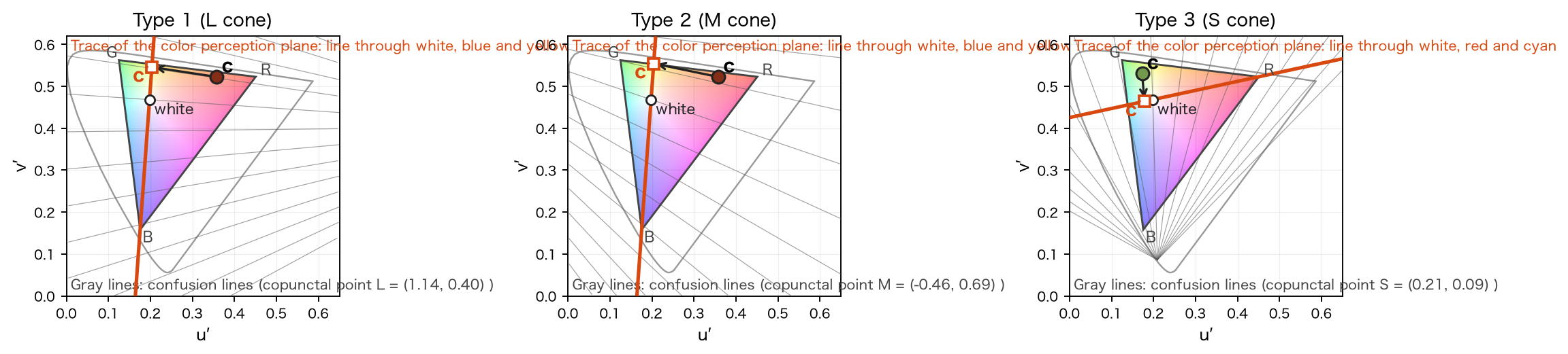
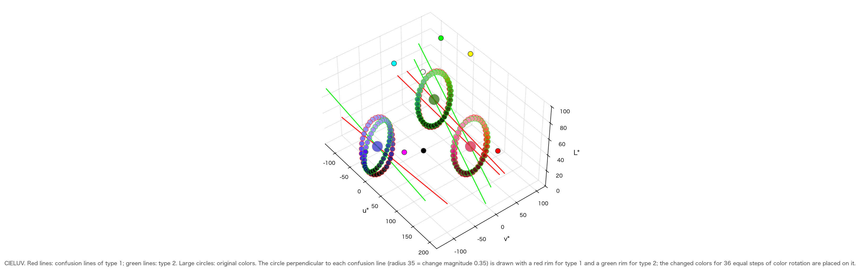
Two colors that differ only in the response of the cone corresponding to the type (L for type 1, M for type 2, S for type 3) are hard for that person to distinguish. In LMS space, such two colors lie on a straight line parallel to the axis of that cone. This line is the confusion line. In XYZ space, the direction of a confusion line is the color $\mathbf{e}$ that stimulates only that cone, that is, the corresponding column of Eq. (12).

The chromaticity of $\mathbf{e}$ (Eq. (16)) is called the copunctal point. On the $u'v'$ diagram, confusion lines are straight lines through the copunctal point. The copunctal points are, for type 1 (L) $(1.1358,\,0.4044)$, type 2 (M) $(-0.4563,\,0.6912)$, type 3 (S) $(0.2090,\,0.0859)$. For types 1 and 2 the copunctal points are far outside the chromaticity diagram and the confusion lines are nearly parallel. The copunctal point of type 3 is below the diagram and its confusion lines fan out (Fig. 1).

6-2. Color perception plane

The whole set of confusion lines is represented by one plane. This is the color perception plane (the single plane of Viénot et al. 1999 [15]). It passes through the origin (black); for types 1 and 2 it passes through the display white, blue and yellow, and for type 3 through white, red and cyan. The plane is determined by the display gamut (sRGB or Display P3) and does not depend on the wavelengths of anchor stimuli. The normal $\mathbf{n}$ is the cross product of the display white $\mathbf{W}$ and the blue (types 1, 2) or red (type 3) primary $\mathbf{B}$, $\mathbf{R}$ (columns of $M$ in Eqs. (5), (7)).

The sRGB values are $\mathbf{n}=(0.8719106,\,-0.7068849,\,-0.1118652)$ for types 1 and 2, and $\mathbf{n}=(-0.2122453,\,0.4307443,\,-0.2102868)$ for type 3. For Display P3 they are $(0.9575963,\,-0.7763530,\,-0.1228586)$ for types 1 and 2, and $(-0.2493665,\,0.5299039,\,-0.2689407)$ for type 3.

Any color $\mathbf{c}$ (XYZ), moved along the confusion line (in the direction $\mathbf{e}$) onto this plane, becomes a color $\mathbf{c}'$ that looks the same to that person.

$s$ is how far $\mathbf{c}$ is from the plane (signed; the red side is $+$). Colors on the plane (white, blue, yellow, etc.) have $s=0$. The difference between $\mathbf{c}$ and $\mathbf{c}'$ is the size of the difference that the person finds hard to distinguish, so using it as an axis lines up the colors the person finds hard to tell apart. In LMS, $\mathbf{e}$ is a unit vector of an axis, so $\mathbf{c}'$ is $\mathbf{c}$ with $s$ subtracted from the LMS component corresponding to the type.

6-3. Chart Angle Method (P)

A fan center $(U_0,V_0)$ is placed on the $u'v'$ chromaticity diagram, and the axis is made from the angle of a color.

The fan center is determined from the two points $\mathbf{E}_1$, $\mathbf{E}_2$ where the trace line of the color perception plane (the line through white and the blue primary (types 1, 2) or the red primary (type 3)) meets the gamut triangle. The XYZ of the two points ($Y=1$) are scaled so that their sum is proportional to white ($s_1\mathbf{E}_1+s_2\mathbf{E}_2=\mathbf{W}$), and the center is the chromaticity of $s_2\mathbf{E}_2-s_1\mathbf{E}_1$ (the harmonic conjugate of white).

$\theta_{\min}$ and $\theta_w$ are the angles of the gamut edges, chosen so that for types 1 and 2 the red primary is $P=0$ and the green primary $P=1$ ($\theta_{\min}$ is the angle of the red primary, $\theta_w$ the difference between the green and red angles), and for type 3 the green primary is $P=0$ and the blue primary $P=1$. The position of white, $P_w$, is obtained from the angle of white by Eq. (25). A plane through the origin is a straight line on $u'v'$, so lines of constant $P$ are radial straight lines from the fan center. The constants are as follows.

The sRGB values agree to within $2.1\times10^{-4}$ with the values hard-coded in 2.21 (centers $(0.214608,\,0.700833)$ and $(0.042256,\,0.434763)$, $\theta_{\min}=0.64566$ and $-0.99599$, $\theta_w=1.49993$ and $2.11836$, $P_w=0.66478$ and $0.36988$) (2.21 rounded the primaries to 4 digits). Types 1 and 2 use the same fan. The $P$ of a given color changes with the color space (the slider is a ratio relative to the gamut at that time).

6-4. Color Appearance Gap Method (A)

Using $\mathbf{c}'$ of Eq. (24), the CIELUV distance between $\mathbf{c}$ and $\mathbf{c}'$ is divided by the original lightness $L^*(\mathbf{c})$. The sign follows $s$.

$\mathrm{Luv}(\cdot)$ is $(L^*,u^*,v^*)$ by Eqs. (16)–(19) (the white is the display white). The difference in lightness ($L^*$) between $\mathbf{c}$ and $\mathbf{c}'$ also enters the distance, so $A$ depends slightly on brightness (differences appear on the blue-violet side).

6-5. Chroma Gap Method (Ch)

The distance of $(a/L,\,b/L)$, that is, Oklab (Eq. (20)) $a,b$ divided by $L$, is used.

As in §5-3, $a/L$ and $b/L$ do not depend on brightness, so $C_h$ is determined by chromaticity alone (changing the luminance $Y$ from 0.001 to 3 changes the value by only $1.7\times10^{-15}$). The confusion line is determined by the cone direction of Eq. (22); Oklab is used only as the yardstick for the distance.

The only difference between A and Ch is the yardstick that measures distance. Both coordinates are converted to the equivalent of $P$ by Eq. (30) of §6-7 and then compared with the zone of Eq. (29).

6-6. Boundaries on the chromaticity diagram

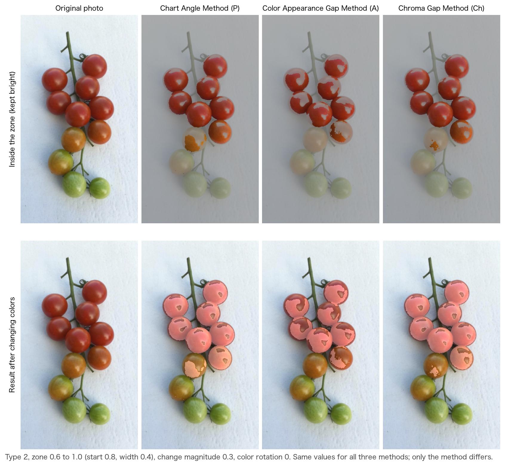
The three methods are compared by where they draw the zone boundary on the chromaticity diagram.

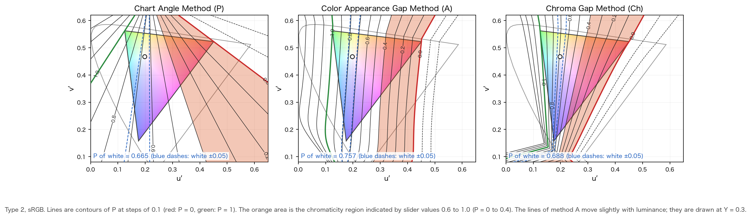
• Chart Angle Method (left): straight lines radiating from the fan center.
• Color Appearance Gap Method (middle): nearly parallel curves. The zone moves like a vertical band from red to green.
• Chroma Gap Method (right): curves close to a fan within the gamut. Lines bend sideways near blue.

The same slider values indicate different colors depending on the method. Figure 9 (§11) shows the results with the same values and only the method changed.

6-7. Zones and slider values

The relation between the slider value $s$ and the axis $P$ is as in 2.21, $s=1-P$ (left end $0$ is the green primary, right end $1$ the red primary; for type 3, blue on the left and green on the right). From the start $a_Z$ (slider value) and the width $w$, the zone is

and a color is inside the zone when its $P$ falls in this range. When "reverse" is on, inside and outside are swapped. $w=0$ means the zone is off (nothing is changed).

For the Chart Angle Method, $P$ of Eq. (25) is used as is. The coordinate $x$ of A and Ch (Eqs. (27), (28)) is converted linearly to $P$, using the primaries themselves (at maximum brightness) of the display as reference.

$a,b$ are determined so that the coordinates $x_{\mathrm{lo}},x_{\mathrm{hi}}$ of the red and green primaries (green and blue for type 3) become $P=0,\,1$: $b=\dfrac{1}{x_{\mathrm{hi}}-x_{\mathrm{lo}}}$, $a=-x_{\mathrm{lo}}\,b$. White lies on the plane, so $x=0$ and the position of white is $P_w=a$. For types 1 and 2, $\mathbf{n}/(\mathbf{n}\cdot\mathbf{e})$ of Eq. (24) is the same for sRGB and Display P3, so the equation for the decision does not change when the color space is switched (only $a,b$ change). For type 3 the plane passes through the red primary, so the values differ with the color space. The values are as follows.

The position of white for the Chart Angle Method is $P_w$ of Eq. (25) (table of §6-3). Within the gamut, $P$ stays within about $0$–$1$ (for Ch the ends coincide with the primaries, so exactly $0$–$1$; for A with type 2, $-0.013$ to $1.001$). Values outside the range are not clipped but compared as they are with Eq. (29).

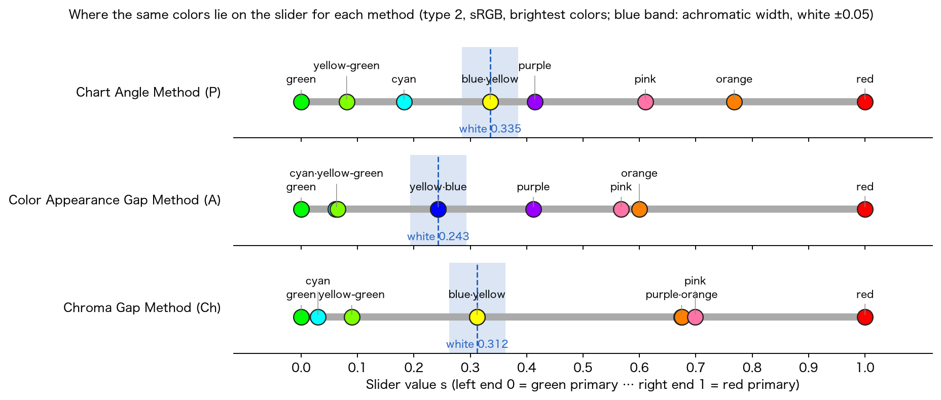
• The positions of the red, green and blue primaries agree for the three methods, so the two ends of the slider have the same meaning.
• A stored value (zone start and width) indicates a different range of colors with the same value when the method is switched.
• The correspondence of A is the value at the primaries (maximum brightness), so it shifts for dark colors (because A depends on brightness). Ch does not shift.

Uniformity of the coordinates. For type 1 and sRGB, when colors are moved along a confusion line, the Oklab distance per unit of coordinate, as a ratio with white as 1 (7 colors: white, gray, skin, yellow, blue-green, blue, dark red), had a max/min of 4.2 for P, 2.7 for Ch and 4.8 for A. Ch narrows the width of blue (the value for blue is 2.35 for P, 0.53 for Ch, 1.18 for A). Only 7 colors and only type 1 were measured.

7. How colors are changed (common to Distinguish and Find)

A color that enters the zone (or the circle around the target color) is moved in CIELUV, confined to the gamut triangle on the chromaticity diagram, and clipped back to the display gamut.

7-1. Direction of the confusion line in CIELUV, $\mathbf{n}_{\mathrm{L}}$

The direction of change is taken different from the direction of the difference the person finds hard to distinguish. First the direction of the color's confusion line within CIELUV is found. The difference between the CIELUV of a color $\mathbf{q}$ (LMS) and that of the color $\mathbf{q}_0$ with the component of the cone corresponding to the type set to $0$ (Eqs. (16)–(19); LMS is returned to XYZ by Eq. (12)) is normalized.

The sign $\sigma$ is the same as in 2.21. For white ($\mathbf{q}=(1,1,1)$) the values are $(0.0234,\,0.9974,\,-0.0680)$ for type 1, $(-0.0754,\,0.9439,\,-0.3215)$ for type 2 and $(0.0115,\,0.0293,\,-0.9995)$ for type 3 (with the 2.21 cones they were $(0.0293,\,0.9992,\,-0.0262)$, $(-0.0643,\,0.9586,\,-0.2773)$ and $(0,\,0.1154,\,-0.9933)$). When the difference is close to $0$ ($<10^{-12}$), $(1,0,0)$ is used.

7-2. Rotation

The rotation that maps the $L^*$ axis $(1,0,0)$ to $\mathbf{n}_{\mathrm{L}}=(n_1,n_2,n_3)$ is given by the following matrix, with $\rho=\sqrt{n_2^2+n_3^2}$, $c=n_3/\rho$, $t=n_2/\rho$, $\varsigma=\sqrt{1-n_1^2}$ (multiplied from the right on a row vector: $\mathbf{v}\mapsto\mathbf{v}R$).

When $\rho<10^{-12}$, $c=1$ and $t=0$ (2.21 divided by 0 and the value was undefined).

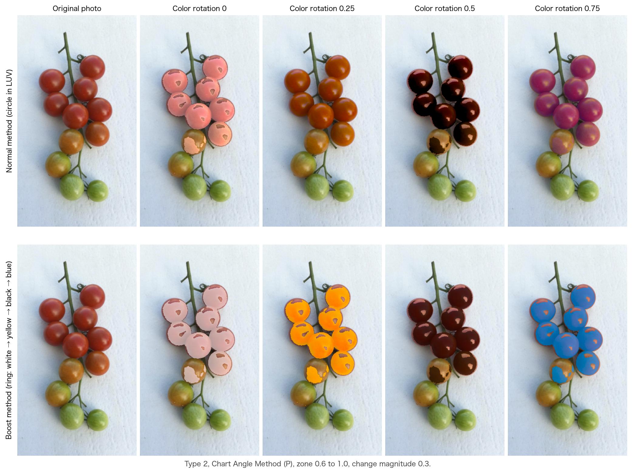
7-3. Normal method: circle in the plane perpendicular to the confusion line

The change vector (CIELUV) is given by the following.

The changed color is $(L^*,u^*,v^*)+\Delta$. $(0,\cos\theta,\sin\theta)$ is a circle perpendicular to the $L^*$ axis, and $R$ turns it into the plane perpendicular to $\mathbf{n}_{\mathrm{L}}$, so $\Delta$ is orthogonal to $\mathbf{n}_{\mathrm{L}}$. The component along the confusion line does not change; only the difference that the person can distinguish increases.

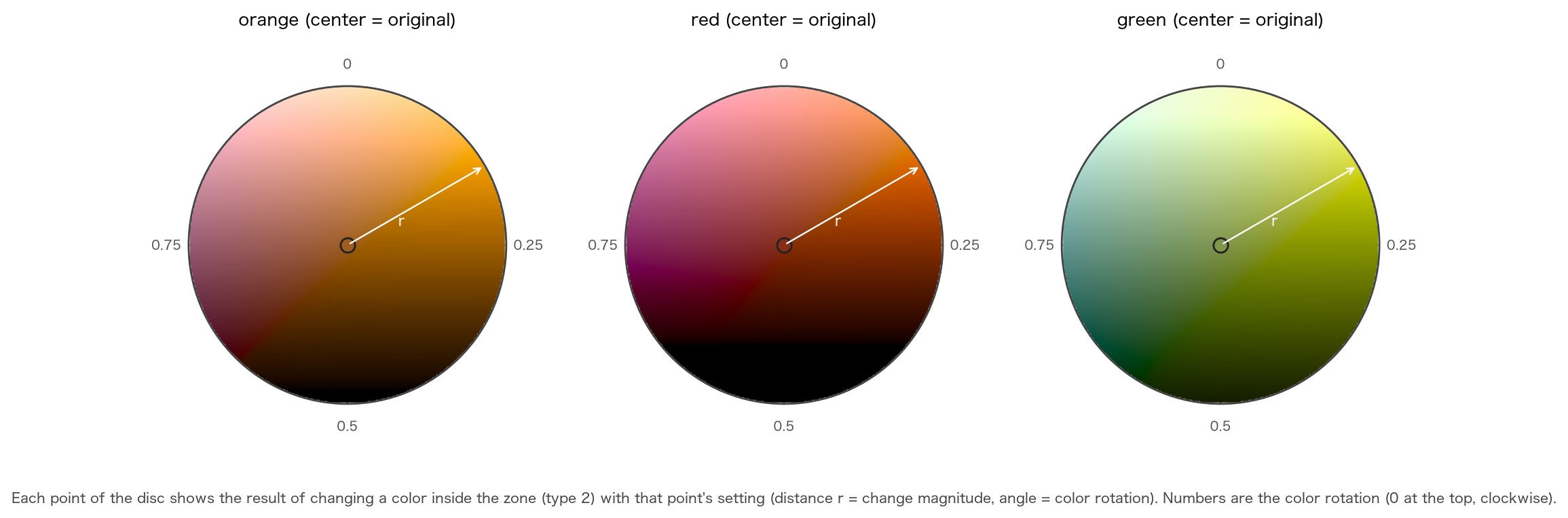
• Radius $=f\cdot100$: the change magnitude $f$ (distance from the center of the 2D slider, $0$ to $0.5$). The constant $100$ is as in 2.21.
• Angle $\theta$: the color rotation $\mathrm{age}$ (angle of the 2D slider; $0$ at the top, one turn clockwise).
• $g$: green-side inversion (§7-4), $0$ or $1$.

The 2D (circular) slider determines the change magnitude $f$ by the distance from the center, and the color rotation $\mathrm{age}$ by the angle. Even at the same position, the way a color changes depends on the original color.

7-4. The π shift on the green side, and the achromatic band

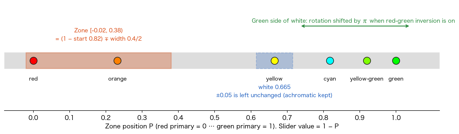
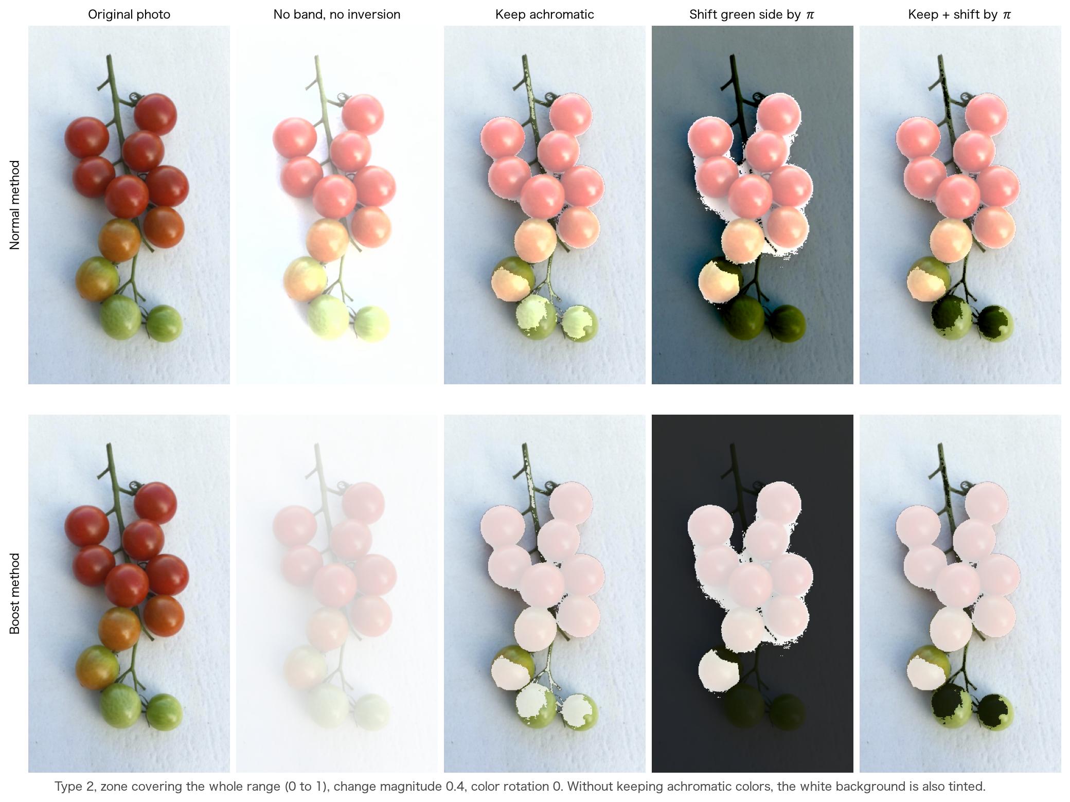
Green-side inversion. When "red-green inversion" is on, a color on the green side of the position of white $P_w$ ($P>P_w$) gets $g=1$, and the angle of Eq. (33) is shifted by $\pi$. Colors on the red side and on the green side move in opposite directions, so the red side and green side can still be told apart after the change. In the boost method, the ring is used shifted by two nodes (§7-5). $P_w$ is the position of white for each method (§6-3, §6-7).

Achromatic band. Colors close to white (gray, a white background) have no hue, so we do not want to change them. When "keep achromatic colors" is on, a color whose $P$ is within $P_w\pm0.05$ around the position of white has its change set to $0$ even if it is in the zone (half of the $0.1$ band width of 2.21).

The apparent width of $\pm0.05$ differs with the method (for A and Ch it is wider on the blue and red sides than for P).

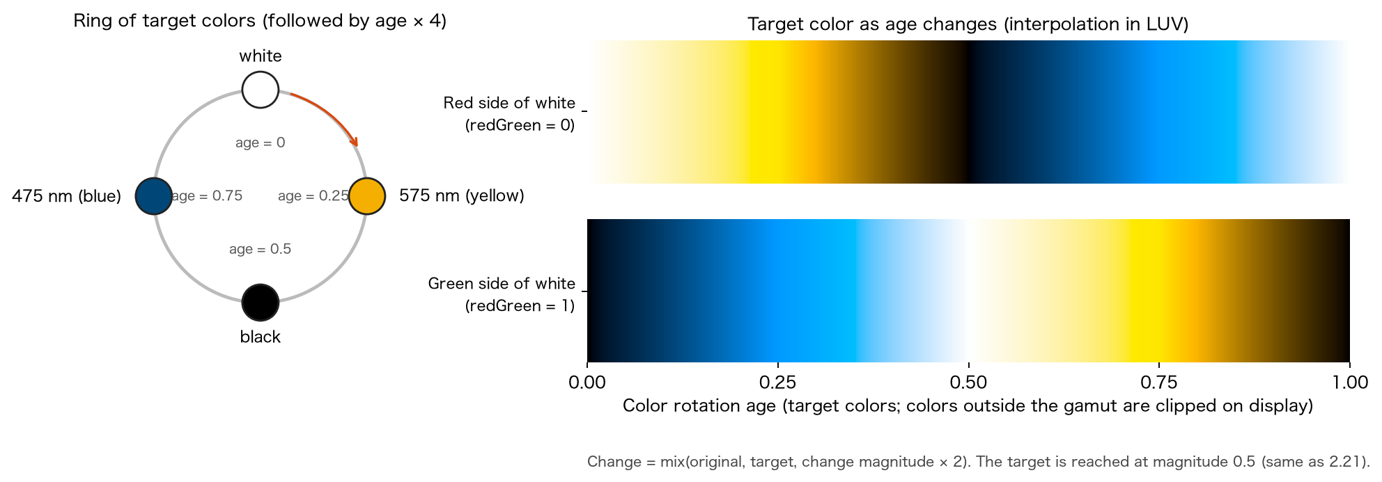
7-5. Boost method

When boost is on (Distinguish only), instead of the circle of Eq. (33), colors are moved toward a target color on a ring. The ring joins four nodes in order: white → 575 nm yellow → black → 475 nm blue (for type 3, 660 nm red and 485 nm blue-green). The nodes are given in $u'v'Y$ (Eq. (16)), and the XYZ of the anchor stimuli use the values $(\bar x_{10},\bar y_{10},\bar z_{10})$ of the CIE 1964 10° color matching functions (JIS Z 8701, Appendix Table 2 [9]).

The CIELUV values of the nodes (Eqs. (18), (19)) are, for types 1 and 2: white $(100,\,0,\,0)$, 575 nm $(96.62,\,77.08,\,116.57)$, black $(0,\,0,\,0)$, 475 nm $(54.02,\,-81.94,\,-115.75)$; for type 3: white $(100,\,0,\,0)$, 660 nm $(29.49,\,145.52,\,17.28)$, black $(0,\,0,\,0)$, 485 nm $(61.46,\,-136.92,\,-29.84)$. Version 2.21 used $L^*=-16$ for the black node.

Let the nodes be $\mathbf{r}_0,\mathbf{r}_1,\mathbf{r}_2,\mathbf{r}_3$ (CIELUV), let the integer part $k$ ($0\le k\le3$) of $4\,\mathrm{age}$ select the node, and the fractional part $\phi$ the position between nodes. The target color $\mathbf{t}$ and the changed color are

($\mathrm{Luv}$ is the CIELUV of the original color). The target is reached at change magnitude $f=0.5$. The upper limit of the 2D slider is $0.5$, so the target is never overshot (above $0.5$ it would extrapolate, but the screen does not produce such values). On the green side ($g=1$) the ring is used shifted by two nodes.

7-6. Confining to the gamut

The CIELUV of the changed color is returned to $u'v'Y$ (inverse of Eq. (19)). When its chromaticity $\mathbf{u}_1=(u',v')$ leaves the gamut triangle of the display (§5-4), the segment from the chromaticity $\mathbf{u}_0$ of the original color toward $\mathbf{u}_1$ is stopped at the point where it reaches the boundary of the triangle. For edge $i$ of the triangle (vertices $\mathbf{a}_i$, $\mathbf{a}_{i+1}$), the signed distance with the inside positive is

($\varpi=\pm1$ is the orientation of the triangle). With $f_0=\max(d_i(\mathbf{u}_0),0)$ and $f_1=d_i(\mathbf{u}_1)$, among the edges with $f_1<0$ take the one with the smallest $t_i=f_0/(f_0-f_1)$ (if no edge is crossed, $t=1$), and let

be the chromaticity and brightness of the changed color. In 2.21, when the original color was on an edge (a saturated color), the intersection test (product of signs) was decided by rounding and the answer differed between single and double precision. This equation computes $t$ after clamping the distance of the original color to $0$ or more, so it gives the same answer regardless of precision (the same as 2.21 for general colors).

Then the display linear RGB (Eqs. (6), (8)) is obtained from the XYZ of the changed color (Eq. (17)), clipped component-wise to $0$–$1$, and encoded (Eq. (2)).

A hue-preserving confinement (lowering brightness while keeping chromaticity) is not used (it is the same component-wise clipping as the strength blending of the Chromatic Vision Simulator).

8. Find colors

Find colors changes only colors close to the target color. It is used when you want to find a specific color (for example, a ripe red fruit) among colors that are hard to tell apart. It does not use the zone axis $P$ but decides by the distance on the $u'v'$ chromaticity diagram.

8-1. Target color

The target color is decided in one of two ways.

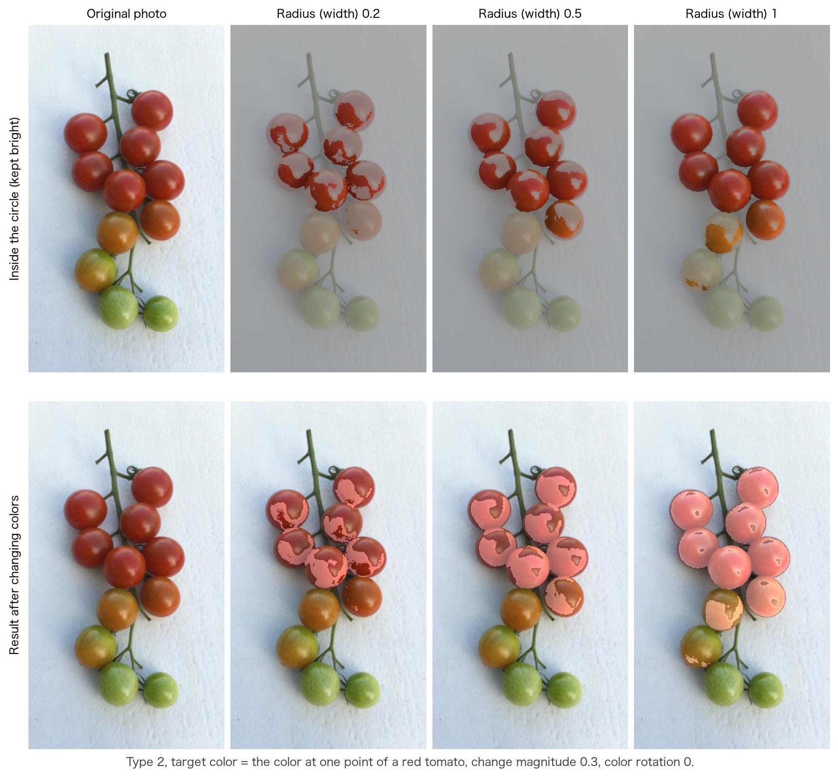
• Tap the image to place the cursor. The color under the cursor (the color averaged smoothly over the surrounding pixels) becomes the target color.
• Choose from the band of 11 basic colors (colors of the Munsell symbols N, R, YR, Y, GY, G, BG, B, PB, P, RP). The cursor moves to the center of that color chip and that color becomes the target color.

The target color (encoded value $\mathbf{c}_s$ of the input) is converted to the chromaticity $\mathbf{s}=(u'_s,v'_s)$ by Eqs. (1), (5) or (7), and (16). Brightness is not considered, so bright and dark areas of the same hue are found alike.

8-2. Range and how colors are changed

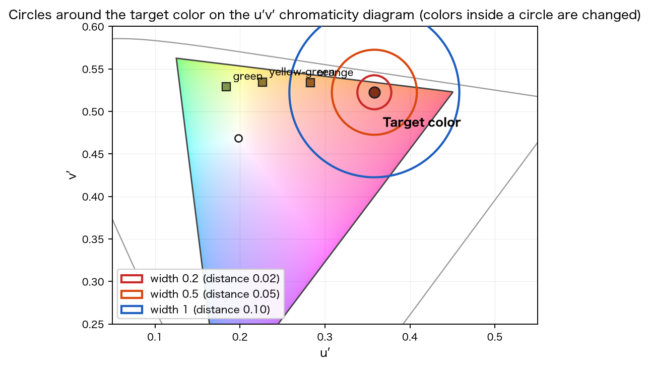
A pixel is changed when its chromaticity $(u',v')$ is close to the chromaticity of the target color.

$w_S$ is the value of the range slider (the radius setting; symmetric about $0.5$, only the distance changes), from $0$ to $1$. At width $1$, colors up to a $u'v'$ distance of $0.1$ (the same value as 2.21) are included. Pixels that satisfy Eq. (39) are changed by the normal method of §7-3 (Eq. (33)) with the change magnitude $f$ (distance on the 2D slider) and the color rotation $\mathrm{age}$ (the same angle). Pixels that do not are left unchanged.

• In Find, the green-side π shift (§7-4), the achromatic band (§7-4) and boost (§7-5) are not used (as in 2.21; boost is for Distinguish only).
• The range is a circle on the chromaticity diagram, so if the target color is close to white, achromatic and pale colors close to white enter the circle.

9. Simulation and display of color names

Simulation simulates how an image looks to a person of type 1, 2 or 3 by the same method as Chromatic Vision Simulator 4.0. The equations and constants are the same; §5 of the theory of Chromatic Vision Simulator 4.0 gives the coefficients of the half-planes (Eqs. (17)–(20)), continuity at the boundary, blending by strength (interpolation in Oklab) and clipping to the gamut. The main points are:

• The color of a pixel is mapped into LMS space, and the component of the cone corresponding to the type is projected onto two half-planes (the folded plane of Brettel et al. [1]) (anchor stimuli of 475 nm and 575 nm for types 1 and 2, and 485 nm and 660 nm for type 3).
• With strength $k$ ($0$ to $1$), the result is blended with the original color by interpolation in Oklab, $\mathbf{o}_k=(1-k)\,\mathbf{o}(\mathbf{q})+k\,\mathbf{o}(\mathbf{q}_s)$ (both ends are first clipped to the display gamut). This only shows the intermediate image between the most severe form of dichromacy and the original image; it does not simulate the color appearance of anomalous trichromacy (mild color vision deficiency).
• The result is confined to the display gamut and encoded.

In Chromatic Glass, the simulation is applied after the change. When the "eye" button is on, the simulation is overlaid on the colors changed by Distinguish or Find, so you can check how the changed colors look to that person. A simulation without any color change is done on the screen of the Simulation function.

The display of color names (the name of the color under the cursor) also works as in Chromatic Vision Simulator 4.0. The colors around the cursor are averaged, and the Munsell value, the systematic color name and the common color name are looked up in a dictionary. See §7 of the theory of Chromatic Vision Simulator 4.0 for details.

10. Overall conversion

The conversion from encoded input $\mathbf{c}_{\mathrm{in}}$ to encoded output $\mathbf{c}_{\mathrm{out}}$ can be written as the composition of §2 to §9. Only the pixels selected by the zone or target-color decision receive the change in CIELUV.

Here $\mathcal{D}$ is decoding (Eq. (1)), $\mathcal{E}$ encoding (Eq. (2)), and $M_{\mathrm{in}}$, $M_{\mathrm{out}}$ the RGB-to-XYZ matrices of the input and the display (Eqs. (5), (7)). $\mathcal{T}$ is the change on XYZ, consisting of the decision (§6 or §8), the change in CIELUV (§7-3 or §7-5), confinement to the gamut triangle (§7-6) and the simulation (§9, when on). For pixels that are not changed, $\mathcal{T}$ is the identity, and the original color is returned.

11. Sample images

The subject is a cherry tomato (the original image on the site). All are for type 2, made with the same equations as in the figures (a copy of the app's reference implementation).

References

[1] H. Brettel, F. Viénot, and J. D. Mollon, "Computerized simulation of color appearance for dichromats", Journal of the Optical Society of America A, vol. 14, no. 10, pp. 2647–2655, 1997. doi:10.1364/JOSAA.14.002647

[2] K. Asada, "Chromatic Vision Simulator", README of the Android source code (appendix: mathematical expressions for color vision simulation), GitHub repository asada0/ChromaticVisionSimulator, 2018, MIT License.

[3] IEC 61966-2-1:1999, Multimedia systems and equipment — Colour measurement and management — Part 2-1: Colour management — Default RGB colour space — sRGB, International Electrotechnical Commission; and Amendment 1:2003.

[4] SMPTE EG 432-1:2010, Digital Source Processing — Color Processing for D-Cinema, Society of Motion Picture and Television Engineers, 2010. doi:10.5594/SMPTE.EG432-1.2010

[5] Apple Inc., "Display P3", Three Component Color Encoding Registry (ICC Registry), International Color Consortium, version 1.0, 2022. https://registry.color.org/rgb-registry/displayp3

[6] T. Smith and J. Guild, "The C.I.E. colorimetric standards and their use", Transactions of the Optical Society, vol. 33, no. 3, pp. 73–134, 1931–32. doi:10.1088/1475-4878/33/3/301

[7] CIE 15:2004, Colorimetry, 3rd ed., Commission Internationale de l'Éclairage, 2004 (including $u'v'$ and CIELUV).

[8] G. Wyszecki and W. S. Stiles, Color Science: Concepts and Methods, Quantitative Data and Formulae, 2nd ed., John Wiley & Sons, 1982.

[9] JIS Z 8701:1999, Colour specification — The CIE 1931 standard colorimetric system and the CIE 1964 supplementary standard colorimetric system, Japanese Standards Association, 1999. Appendix Table 2 (spectral chromaticity coordinates of the X10Y10Z10 system; the source of the 10° anchor stimuli).

[10] R. W. G. Hunt and M. R. Pointer, "A colour-appearance transform for the CIE 1931 standard colorimetric observer", Color Research & Application, vol. 10, no. 3, pp. 165–179, 1985. doi:10.1002/col.5080100306

[11] M. D. Fairchild, Color Appearance Models, 3rd ed., John Wiley & Sons, 2013. doi:10.1002/9781118653128

[12] C. Poynton, Digital Video and HD: Algorithms and Interfaces, 2nd ed., Morgan Kaufmann, 2012.

[13] Colour & Vision Research Laboratory, UCL Institute of Ophthalmology, "CIE 1931 2-deg XYZ color matching functions (ciexyz31_1.csv)" and "CIE 1964 10-deg XYZ color matching functions (ciexyz64_1.csv)", http://cvrl.ioo.ucl.ac.uk/cmfs.htm

[14] B. Ottosson, "A perceptual color space for image processing", blog post, 23 December 2020, https://bottosson.github.io/posts/oklab/

[15] F. Viénot, H. Brettel, and J. D. Mollon, "Digital video colourmaps for checking the legibility of displays by dichromats", Color Research & Application, vol. 24, no. 4, pp. 243–252, 1999.