Theory of the Eye Age Simulator
1. Overview
This paper formulates, with optical equations, how the Eye Age Simulator reflects "how aging and cataract change vision" in an image, and gives the sources of the numbers it uses. It describes in turn the three changes that happen to light inside the eye (absorption by the lens, scattering, and blocking by opacities), the pupil diameter, and the treatment of strong light that a screen cannot display.
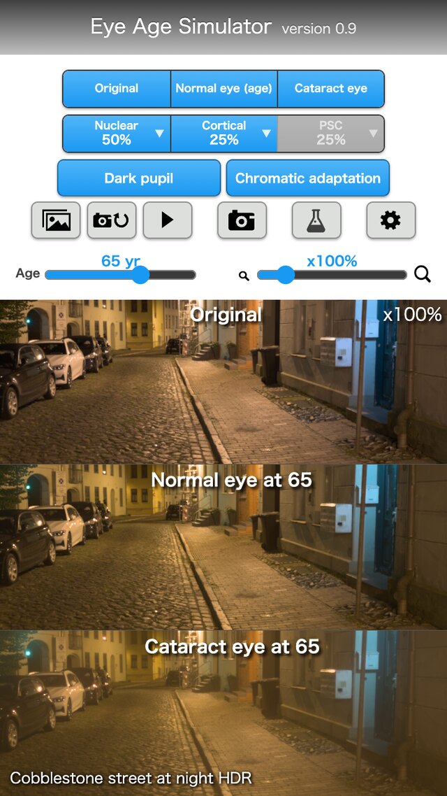
The screen can show three panels side by side.
| Panel | Content | Sections |
|---|---|---|
| Original image | The image without processing | §2 |
| Normal eye of the chosen age | The image with the increments from a 20-year-old eye (lens yellowing, light scatter) reflected | §2, §4, §6 |
| Cataract eye | The normal eye of the chosen age, with the contributions of the opacities of the cataract type (nuclear, cortical, posterior subcapsular) and its progress reflected | §7, §8, §11 |
Some numbers have been confirmed in papers and standards; others were set as guides where no literature was found. §14 distinguishes the two, one parameter at a time. This app cannot be used for diagnosis, treatment or visual acuity tests (§13).
Key point: The calculation that brings the retinal image of the viewer, who looks at the screen, close to the retinal image that the target eye forms from the real scene is defined as equations.
1-1. Assumptions
The following hold throughout this paper.
- 1. Image: an 8-bit sRGB image is converted to linear light with the transfer function [10]. White is . An HDR image (such as Ultra HDR) is used by restoring the HDR linear light from the base SDR picture and the gain map (§3).
- 2. The viewer's eye: the image on the screen reaches the retina through the viewer's own eye. The viewer's eye is taken as the reference eye, and by default is assumed to be a young normal eye of 20 years (§2).
- 3. Color and wavelengths: color is handled with cone signals (LMS) and Oklab (§4, §10). The core of the point spread function is calculated at three representative wavelengths for R, G and B (, and nm; at most nm from the dominant wavelengths of the sRGB primaries for the 2° observer) (§7).
- 4. Pupil: decided from the brightness of the field, with both eyes adapted (§5).
- 5. Cataract: expressed with three types (nuclear, cortical, posterior subcapsular) and a progress from to . The shapes and sizes of opacities are guides set with reference to the definitions of clinical classifications, not values fitted to them (§7, §11).
- 6. Scene brightness: the "white luminance" of a sample image (how many cd/m² the image white stands for) is set for each scene. An HDR image depends on the original exposure and has no absolute luminance. For night scenes with street lighting, the median luminance of the image is matched to the average road-surface luminance of a road lighting class (§3-3).
- 7. Corrected state: the refractive blur that glasses can correct (myopic shift) is not included in the general settings. The app deals with how cataract looks in the corrected state (§12).
- 8. Outputs not provided: visual acuity, contrast sensitivity and visual field are not output.
1-2. Notation
| Symbol | Meaning | Section |
|---|---|---|
| Linear light of the scene (each RGB component, white ; may be HDR) | §2, §3 | |
| Light displayed by the screen (linear, white is the upper limit) | §2 | |
| , | Retinal images of the target eye and of the viewer's eye | §2 |
| , , | Point spread function (PSF), its core (sharp part), and the distribution of wide scatter | §2, §6, §7 |
| , , , | Lens transmittance, ratio of transmittances per wavelength, cone-wise ratio, ratio with color adaptation | §4 |
| , , , | Difference of age factors , degrees of adaptation of the L and M cones and of the S cones (always with a subscript), brightness correction factor | §4 |
| , , | Cone signals (LMS, white ), input and output matrices | §10 |
| , , | Oklab lightness and two color axes, chroma, hue | §10 |
| , | Chosen age, viewer's age (default ) | §2, §4 |
| , | Optical density, wavelength (nm) | §4 |
| , , | Straylight parameter (deg²/sr), its common logarithm, scatter multiplier (normal ) | §6 |
| Component above white ( for each channel of linear RGB) | §2, §3 | |
| , , | Angle from the light source (degrees), illuminance at the eye, equivalent veiling luminance | §3, §6 |
| Pupil diameter (mm; no subscript) | §5, §7 | |
| , | Amplitude of the pupil function, optical path difference | §7 |
| , | Depth of an opacity (from the pupil plane, mm), field angle | §7 |
| Fraction of the pupil covered by an opacity | §8 | |
| , | Gain (), gain map value | §3 |
| Convolution | §2 |
Key point: The equations below express light as linear light (white ), angles in degrees, and lengths in mm.
1-3. Processing flow
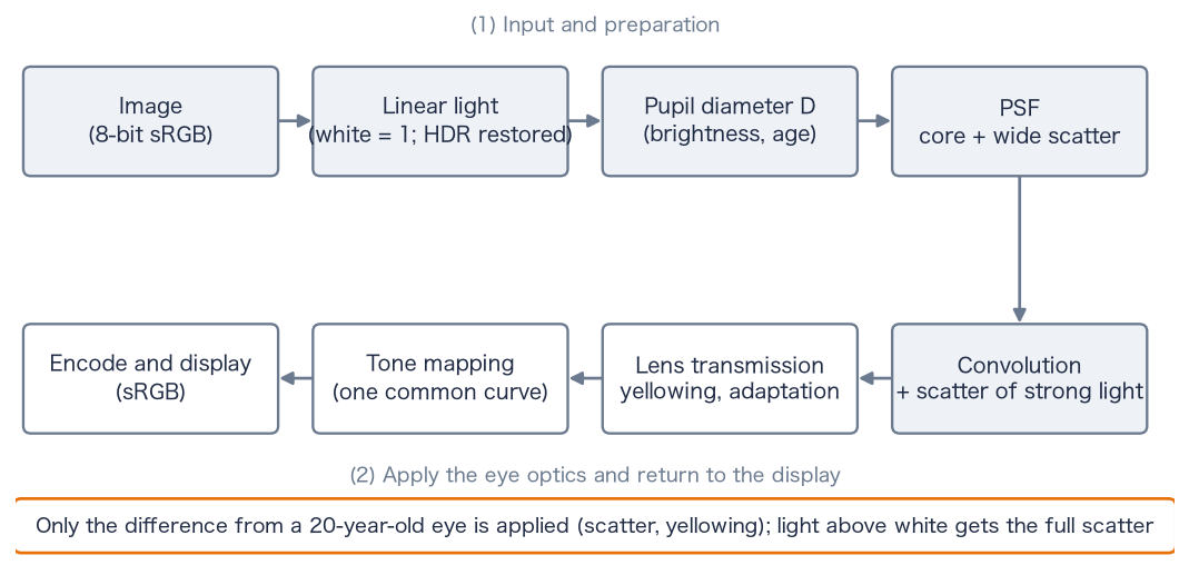
image ──(§3)──▶ linear light L (white = 1; restored if HDR)
   mean image brightness ──(§5)──▶ pupil diameter D
   D, age, opacities ──(§7)──▶ core PSF (diffraction, opacities) and weights of the wide scatter (§6, §8)
L ∗ (core + increment of the wide scatter)  +  scatter of light above white (§2-5)
   ──(§4, §10)──▶ in LMS, reflect the cone-wise ratio of transmittances (yellowing, color adaptation)
   ──(§10)──▶ tone mapping in Oklab (hue kept) ──▶ return to the display color space, encode and display
1-4. Structure of the eye and the parts to which the parameters correspond
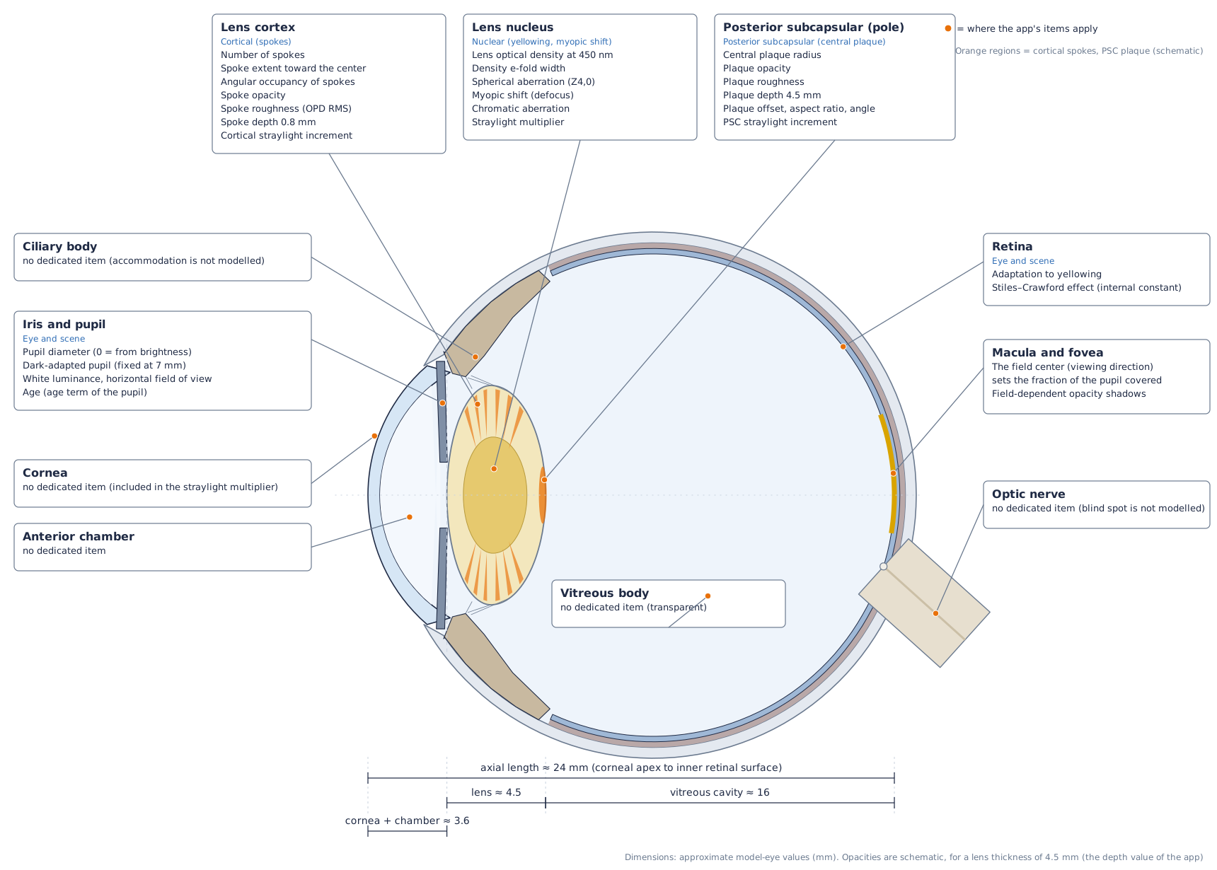
The axial length (corneal apex to the inner surface of the retina) is about mm. It is divided into the cornea and anterior chamber (about mm), the lens (about mm at 50 to 60 years; about mm at 20 years and mm at 70 years), and the vitreous cavity (about mm) [13][14]. The pupil lies just in front of the anterior surface of the lens, and this paper calls this plane the pupil plane. The nucleus of the lens is its central part, the cortex is the outer layer around the nucleus, and the posterior capsule is the thin membrane that encloses the back of the lens.
Key point: The parameters of the app correspond roughly to three parts: the lens (nucleus, cortex, capsule), the pupil and the retina.
1-5. Cones of light and the position of opacities
Light emitted from one point of the scene enters through the whole pupil, is refracted by the lens, and converges to one point on the retina. This bundle of light is called a cone of light in this paper. The diameter of its cross-section equals the pupil diameter at the pupil plane and becomes smaller toward the retina. At a plane at distance from the pupil plane, the diameter is approximately
where is the distance from the pupil plane to the retina.
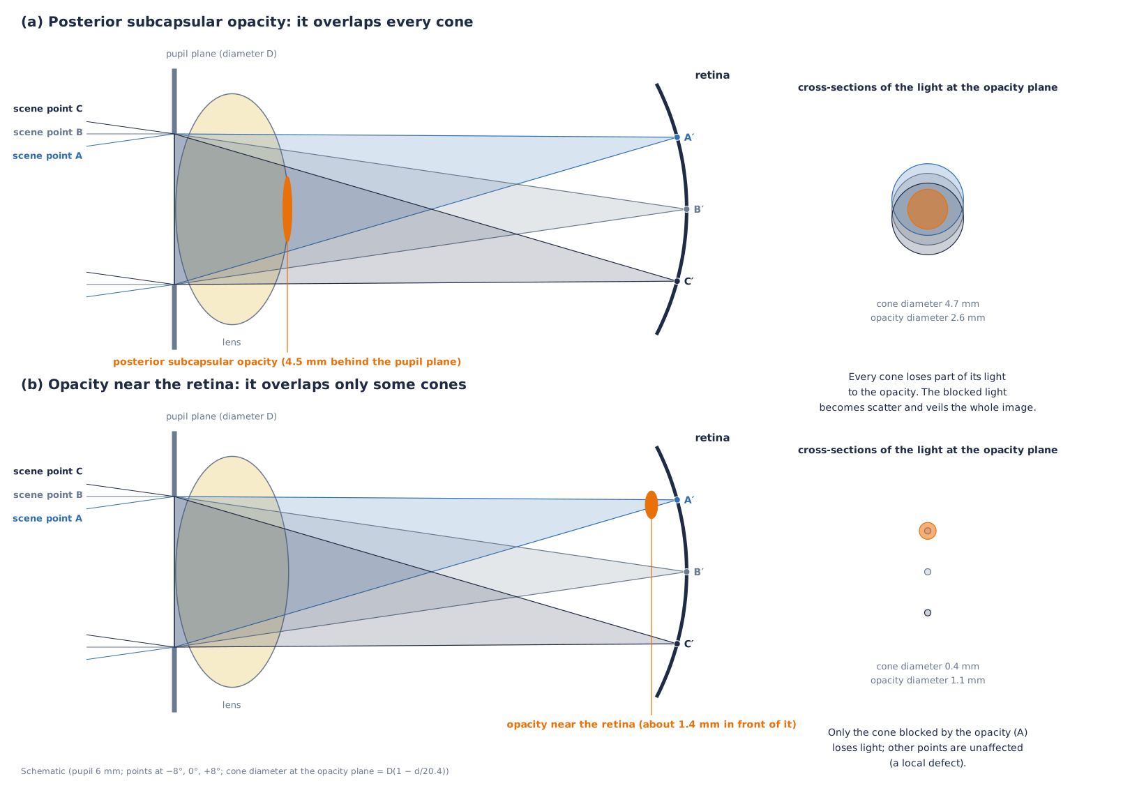
A posterior subcapsular opacity, at the center of the back of the lens, overlaps the cross-section of every cone. Part of the light of every point of the scene is blocked by the opacity, and the blocked light goes to scatter. The whole image therefore becomes hazy. For an opacity near the retina, the cross-sections of the cones are small, and only the light of the points blocked by the opacity is lost. The difference—posterior subcapsular cataract produces an overall haze, whereas an opacity near the retina produces a local defect—is explained by this geometry. A nuclear opacity lies throughout the lens and every cone passes through it, so it acts uniformly on the whole image.
Key point: Whether an opacity acts on the whole image or on a part of it is determined by its depth (its distance from the retina).
1-6. The three types of cataract
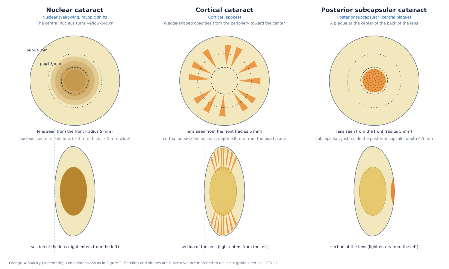
Nuclear cataract is a yellow-brown opacification and coloring of the nucleus at the center of the lens. Cortical cataract is an opacity in the cortex that appears as spokes [15]; this app represents it as wedges extending from the periphery toward the center (§7-3). Posterior subcapsular cataract is a plaque-like opacity just beneath the posterior capsule at the posterior pole of the lens [15].
Key point: The three types differ in position and shape inside the lens, and therefore differ in their effect on the image.
2. Reflecting the increments over the reference eye
This section formulates how the image on the screen should be made so that the viewer's retinal image approaches the retinal image of the target eye.
2-1. Purpose and the reference eye
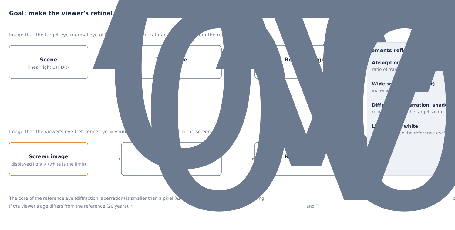
The image on the screen reaches the retina through the viewer's eye. The viewer's eye already applies diffraction, the focus difference between wavelengths, scatter and lens absorption to the image. If the optics of the target eye (the normal eye of the chosen age, or a cataract eye) were laid over the image by calculation, the viewer's part would be counted twice and the image would be degraded compared with the original.
So the viewer's eye is taken as the reference eye and assumed to be a young normal eye of 20 years. Only the part by which the target eye exceeds the reference eye is reflected in the image.
2-2. Formulation of the retinal images
Let be the linear light of the scene and the light displayed by the screen. With the PSF and lens transmittance of the target eye, and the PSF and transmittance of the reference eye, the retinal images are
The required is the image that satisfies .
The PSF is expressed as the sum of a sharp core and a distribution of wide scatter .
The ratio of lens transmittances is defined as follows (§4).
2-3. Reflecting the increments
If the core of the reference eye is assumed to be sufficiently smaller than a pixel (§2-4), then . The following then gives .
Here is the increment of the wide scatter. Scatter is an addition of light, so it can be expressed by adding the increment. Absorption is a multiplicative effect, so it is expressed by the ratio of transmittances . Substituting Eq. (5) into (2) and approximating gives . The neglected terms are second-order terms such as products of scatter with scatter.
2-4. Treatment of diffraction and aberration (the core)
Blur such as diffraction and aberration, unlike scatter, cannot be reduced to an increment by a calculation (deconvolution). So the core is reproduced with the values of the target eye. The core of the viewer's eye also acts, so diffraction is duplicated, but in ordinary display its size is smaller than a pixel. The full width at half maximum of the Airy disk, for wavelength and pupil diameter , is
It is about arcmin for mm and nm (about arcmin for mm). When the angle of a pixel (field of view ÷ number of pixels) is larger than about arcmin (about arcmin for a field across pixels), the effect of the duplication hardly appears. Only when the angle of a pixel is about arcmin or less (about times as many pixels or more for the same field of view) does the viewer's own eye make the image softer.
2-5. Light above white
The screen cannot display light brighter than white (SDR ). For strong light such as headlights, street lamps and the sun, the scatter that this light would produce in the viewer's eye is not contained in the displayed image. Eq. (5) applies when the light of the scene falls within what the screen can display.
Let the component above white be for each channel of linear RGB. For , the scatter of the reference eye is also reproduced. What the screen cannot display is the part of each channel above , so the judgement is made per channel (light such as a red tail lamp, whose luminance is below but whose R exceeds , is not missed).
The third term supplements the scatter that the viewer's eye cannot apply to light that was not displayed. The supplementing light is exactly the part of each channel that the screen could not display (the part above of the RGB restored with the gain map). With this term, the scatter for becomes . The part above white is displayed clipped to white on the screen, so the supplemented scatter is not counted twice.
2-6. When the viewer differs from the reference eye
When the viewer is elderly, the viewer's eye differs from the reference eye ( years), and differ from the reference, and the approximation breaks down. If the viewer's age is specified, and are replaced by the values at age . When is higher than the target age , the increment becomes negative. The increment of scatter is limited below at , and for yellowing the ratio of transmittances exceeds , which returns toward more blue. For a viewer who is actually 50, with left at the default and a chosen age of 65, the straylight parameter reaching the viewer's retina is deg²/sr, about more than the target (Eq. (32)). With specified, it matches the target.
Key point: Only the increment of the target eye over the reference eye is reflected in the image. Scatter is added as an increment, absorption is expressed by the ratio of transmittances, and diffraction and aberration are reproduced with the values of the target eye. Light above white is reproduced including the scatter of the reference eye.
3. Encoding of images and restoring HDR
This section gives the equations that obtain linear light from encoded values, and that restore HDR light.
3-1. Transfer function and luminance
The conversion from the 8-bit encoded value (; pixel value ) to linear light uses the sRGB transfer function [10][16].
The inverse conversion for display is
The luminance is a linear combination of linear RGB: with the coefficients of ITU-R BT.709 [17] for sRGB, and in general the second row of the matrix of the capture color space (§10-1).
3-2. Restoring HDR with the gain map
In an Ultra HDR JPEG, the first JPEG is the SDR picture (the base picture), and the second JPEG (pointed to by the MPF) is the gain map. The gain is determined from the gain map value ( to ) [8].
The HDR linear light is restored from the linear value of the base SDR as follows (for each RGB channel, as a multiple of white ).
and are the minimum and maximum gain, is the gamma, and is the offset. They are read from the XMP hdrgm or from the binary of ISO 21496-1 [9]. The equation of the specification includes a weight according to the display capability of the screen, as [8]. The purpose of this app is to restore the light of the scene, so it uses . A photo without a gain map is handled as (left as SDR).
Samples are made with a 3-channel RGB gain map (8 bits, the same size as the base picture, ) (the source images of the samples are [11]; is a choice of this app, different from the default of the Android specification [8]). The base picture is an SDR in which the part of the largest channel above the knee is moved toward white.
3-3. Why the true intensity of light is needed
Straylight inside the eye is proportional to the product of the luminance and the solid angle of the source (the illuminance at the eye). From the CIE equation (§6), the luminance of the haze at an angle from the source is
is the straylight parameter of §6, a constant independent of angle. The haze is determined by the product of the area and the luminance of the source, and does not depend on its apparent shape.
An SDR image is cut off at white (), and a white sheet of paper, a headlight and the sun are all , so cannot be known from the image. In the night-road headlight sample, the luminance of the lamp disk is about times white (luminous intensity cd, distance about m, illuminance at the eye about lx). If this light is set to the SDR , becomes about and the haze is underestimated by about . In the street-light sample, the brightest position (the 99.95th percentile) is tens to hundreds of times white. The gain map restores this intensity of light, and it is used for in Eq. (7).
The absolute level of the image (white luminance ) of night scenes with street lighting is set by matching the median luminance of the image to the average road-surface luminance of a road lighting class. The classes and average illuminances are the P classes of EN 13201-2:2015 [48] (aligned with the classes of CIE 115:2010 [47]): P2 lx, P3 lx, P4 lx, P5 lx. The road-surface luminance is obtained from the illuminance with the average luminance coefficient cd/m²/lx of the standard road surface R3 of CIE 144:2001 [49].
is the median luminance of the image with white ( to for night scenes). The white luminances of the samples are for the cobblestone street at night (P3), for the plaza at night (P2), for the night city square (P2), for the night alley (P4), for the park at night (P5) and cd/m² for the snowy night (P5). Scenes without lamps (moonlight), dusk, and the headlight photograph (lamps composited from luminous intensity and distance) are outside this method. Eq. (13) is linear in , so the spread of haze is determined by the ratio of lamp to road surface and does not change when the absolute level of the image is changed uniformly. The absolute level changes the pupil diameter (§5) and the degree of adaptation (§4-3).
3-4. Kinds of input images
- Ultra HDR JPEG (XMP hdrgm) and ISO 21496-1 JPEG: restored with Eqs. (11) and (12).
- Apple's own JPEG format (the second picture of the MPF and the headroom in the MakerNote): a reading process exists, but it has not been confirmed with real photos.
- HEIC: not read directly. For a new iPhone HDR photo, the ISO 21496-1 gain map remains when Safari converts the HEIC to JPEG, and it can be read by the route above.
Key point: By restoring the true intensity of light from the SDR picture and the gain map, the scatter caused by light above white can be reproduced.
4. Lens transmission and color adaptation
This section expresses the absorption of the lens as a spectral optical density that depends on age and cataract, and defines the cone-wise ratio of transmittances and color adaptation of the von Kries type.
4-1. Optical density of the lens
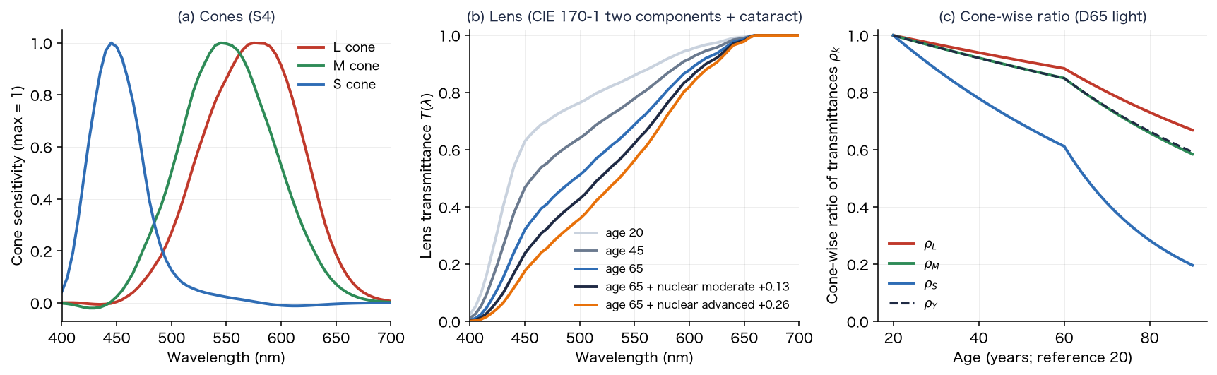
The transmission of light through the lens is expressed with the optical density at wavelength (the negative of the common logarithm of the transmittance). CIE 170-1:2006 [45] expresses the density of the lens and other ocular media as the sum of a component that increases with age and an age-independent component (standard for 32 years, small field; equations and tables in [35]). The density of a normal lens at age is
At nm, and ; the density is at 20 years and at 65 years. is large below nm ( and at nm) and does not change with age. The increase of density at nm with age is per decade up to years and per decade above , close to the and of Pokorny et al. [12]. agrees with the 32-year table of Stockman, Sharpe and Fach [46] at nm and above.
The increment of nuclear cataract is given the same spectral shape as the age-dependent component . Delahunt et al. [4] fitted the density of cataractous lenses with the spectral shape of the aging component (the of Pokorny et al.).
is the increment at nm: early , moderate , advanced (table in §14-2). The moderate stage was set so that, for a 70-year-old eye, it matches the measurement of Delahunt et al. [4] that cataractous lenses (grades 2 to 3+) reduced light intensity by about (the value giving luminance transmittance is ). The early and advanced stages are about and times the moderate stage (an assumption of this app).
4-2. Age and cataract parts, and the cone-wise ratio of transmittances
The difference in optical density between the target eye and the reference eye (age ) is the sum of the age part (the difference of age factors multiplied by ; cancels) and the cataract part.
is the ratio of transmittances per wavelength (Eq. (4)). The colors of the image are handled as cone signals LMS (§10), so the ratio is converted to cone-wise values (). The spectral sensitivity of cone is obtained by applying the cone matrix (cone system S4 [41]; §10-1) to the CIE 1964 10° color-matching functions . The white of the display is equivalent to D65, so the weighting uses the spectral distribution of the standard illuminant D65.
The integrals are sums over to nm at nm steps. After the lens, the cone signals become . This approximation is exact for narrow-band light; for broad-band light it has an error because the weights of the cone responses change with the spectrum.
| Condition (reference 20 years) | ||||
|---|---|---|---|---|
| 40 years | ||||
| 65 years | ||||
| 80 years | ||||
| 65 years + nuclear early () | ||||
| 65 years + nuclear moderate () | ||||
| 65 years + nuclear advanced () |
4-3. Color adaptation (von Kries) and its limits
Light that passes a yellowed lens loses blue and takes a yellowish tint overall. After a long period of cataract, the brain adapts to this bias and becomes less aware of the yellow tint. Adaptation, however, has limits. Delahunt et al. [4] measured the "color that looks achromatic" of 4 people (aged to ) who had the yellowed lens removed by cataract surgery, from before surgery for up to 1 year. After surgery, the achromatic setting first moved strongly toward yellow, and it returned largely over about 3 months (no proportion is given), but it did not return completely. The remaining bias was in the yellow direction (the S-cone axis), and the authors state that it is unlikely that all of the change is discounted when little short-wavelength light reaches the retina. The usual yellowing of aging is compensated well, but incompletely for the densest lenses (Kraft and Werner [7]).
This adaptation is expressed by a von Kries-type transform that changes the gain of each cone, with separate degrees of adaptation for the L and M cones and for the S cones. Let be the ratio of lens transmittances for the luminance of white.
The degree of adaptation of the L and M cones, , uses the CIECAM02 equation for the degree of adaptation [44]. is the luminance of the adapting field (cd/m²), taken as of the white luminance of the image , with an average surround ().
is for a night street (), indoors () and outdoors in daylight (). The degree of adaptation of the S cones, , is an assumption based on the "incomplete compensation" of Delahunt et al. and Kraft and Werner; there is no numerical literature value (§14). is the state before adaptation and is complete adaptation.
4-4. Adaptation to brightness
Lens absorption lowers the retinal illuminance, and the visual system also adapts partly to a drop in brightness. The app multiplies by the following correction factor , computed from the luminance of the adapted ratio of transmittances.
means complete compensation and means none. is the same factor for all components, so it does not change chromaticity or hue.
4-5. The 3×3 matrix that reflects the lens
The transform that reflects the lens, color adaptation and brightness correction is a diagonal matrix on cone signals, combined with the input and output matrices (§10; Eq. (50)) into a 3×3 matrix on linear RGB.
White is mapped to ( is included only once, in the diagonal of Eq. (25)); for a normal 65-year-old eye (reference 20 years, ) it is . The appearance of white (D65) is as follows (Oklab hue and chroma, before tone mapping).
| Condition | With adaptation (hue, chroma) | Without adaptation (hue, chroma) |
|---|---|---|
| Normal eye, 20 years | achromatic | achromatic |
| Normal eye, 65 years | , | , |
| Normal eye, 80 years | , | , |
| 65 years + nuclear early | , | , |
| 65 years + nuclear moderate | , | , |
| 65 years + nuclear advanced | , | , |
With adaptation, a bias toward yellow (hue around ) remains. Without adaptation, white shifts toward yellow-orange (hue to ).
Key point: The absorption of the lens is reflected in LMS as the cone-wise ratio of transmittances , from the sum of the age part (the age-dependent component of the two components of CIE 170-1) and the cataract part (the same spectral shape). Color adaptation uses the CIECAM02 degree of adaptation for the L and M cones and an incomplete value () for the S cones, so a yellow tint remains.
5. Pupil
This section gives the equations that decide the pupil diameter from the brightness of the image and from age.
The pupil diameter is decided from the luminance (cd/m²) and the field area (deg²) with the unified formula of Watson and Yellott [1]. For adaptation with both eyes, .
The pupil diameter is limited to to mm. The field area is the width × height (in degrees squared) of the field of view of the image (default ), and is the mean luminance of the image multiplied by the white luminance of the image. The "dark-adapted pupil" is fixed at mm. For camera video, the pupil diameter changes as a first-order lag with a time constant of s, to avoid sudden flicker.
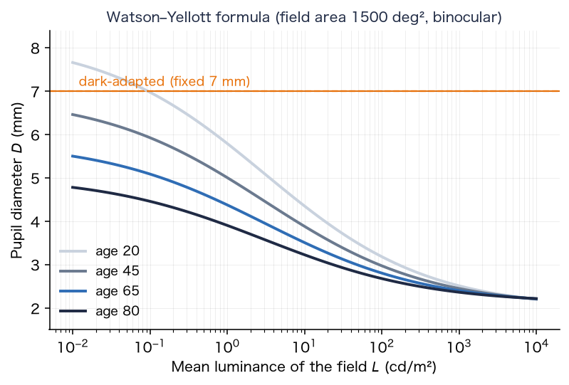
Key point: The pupil diameter is decided by the brightness of the image and by age. The larger the pupil, the smaller the diffraction and the larger the contribution of opacities.
6. Straylight (scattering of light)
This section quantifies the amount of light scattered into wide angles inside the eye (straylight), with the CIE equation and clinical measurements.
6-1. The straylight parameter
Straylight is expressed with the straylight parameter . At angle from a point source, it is defined as the ratio of the luminance of the equivalent veiling light to the illuminance that the source produces at the eye.
One equation of the CIE standard glare observer [2][34] is the Stiles–Holladay equation with an age correction. It is valid for from about to .
At 65 years, (), and at 20 years (), so the value at 65 years is about times that at 20 years.
6-2. Angular distribution and the fraction of light spread
The app uses Eq. (29) from to , keeps it constant inside , and lets it fall as outside . The distribution of wide scatter per steradian is
The fraction of light spread, integrated over solid angle up to (including the constant part inside ), is
For a normal 65-year-old eye, .
6-3. Multiplier for cataract, and the part of the viewer's eye
The straylight of a cataract eye is expressed by multiplying the age term by a multiplier (normal ), as a difference from the reference eye.
For a 65-year-old eye, . The multiplier is set by the tables of §8 and §11.
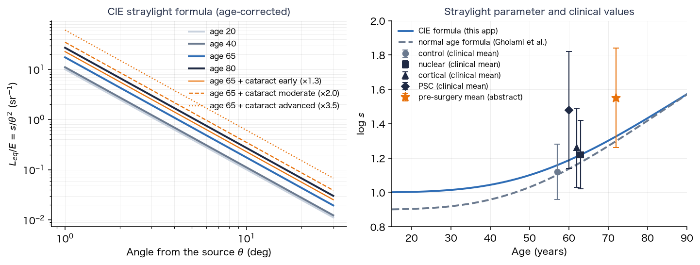
6-4. Comparison with clinical values
The values of Table 4 (measured with the C-Quant) of Gholami, Reus and van den Berg (2017) [3] are as follows.
| Group | Age (mean) | (mean ± SD) |
|---|---|---|
| Control | 57 ± 8 years | 1.12 ± 0.16 |
| Nuclear cataract | 63 ± 9 years | 1.22 ± 0.20 |
| Cortical cataract | 62 ± 8 years | 1.26 ± 0.23 |
| Posterior subcapsular cataract | 60 ± 8 years | 1.48 ± 0.34 |
The number of eyes is for the control, for nuclear and for posterior subcapsular (a pool of five studies). The normal age formula of the same paper is
It gives at 65 years, close to the of Eq. (29). At the control mean age of 57 years it gives , which agrees with in the table. For patients undergoing surgery, the preoperative mean is , and the branch point at which the probability that surgery improves vision is is a corrected visual acuity of logMAR and (van der Meulen et al. [5]).
Key point: Straylight is expressed by an age term and a cataract multiplier, with for a normal 65-year-old eye. The stages of this app are matched to the increments of the clinical means (nuclear , cortical , posterior subcapsular ) over the normal values at the ages of the groups (§11).
7. Point spread function (PSF)
This section shows how the blur of the image of the eye (the spread of the image of a point source) is calculated from the pupil function.
The PSF is made in two parts, the core (diffraction and the shape of the opacities) and the wide scatter (§6, §7-5), and convolved with the image (linear light).
7-1. Pupil function and core
The squared magnitude of the Fourier transform of the complex amplitude in the pupil plane is the core PSF.
is the amplitude (zero outside the pupil) and is the optical path difference. With no opacity, a circular pupil and no aberration, the PSF is the Airy disk. It is calculated for each wavelength (, and nm) and normalized to a total of .
7-2. The Stiles–Crawford effect and aberration
The Stiles–Crawford effect is the lower retinal sensitivity to light that is farther from the center of the pupil. The intensity falls as ( is the distance from the pupil center in mm, ), so the amplitude is its square root.
Spherical aberration is expressed with the Zernike polynomial . With (normalized to the radius of a mm pupil),
is the RMS value (µm) for a mm pupil, set to , and µm for early, moderate and advanced nuclear progress. Nuclear cataract has been reported to shift spherical aberration toward negative values [22][23]. The refractive blur (myopic shift) and chromatic aberration are added to as defocus at wavelength (in the general settings the myopic shift is , and chromatic aberration is not added, being the same as in the reference eye).
is the myopic shift (D) and is the longitudinal chromatic aberration (D), in the form of the equation of Thibos et al. [18].
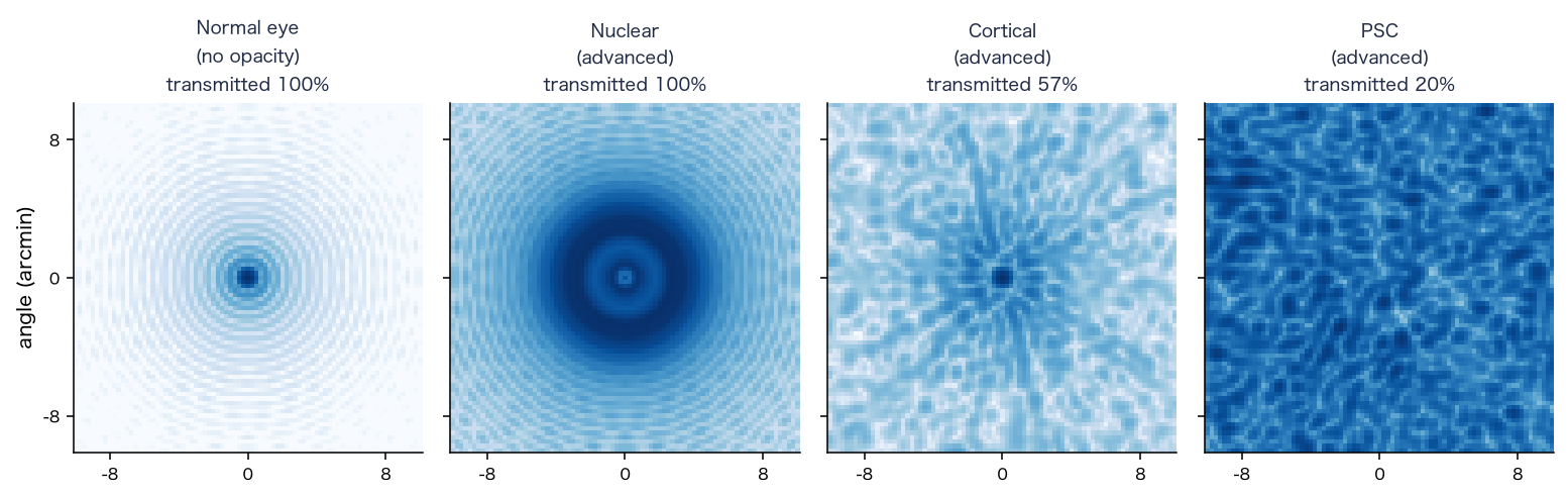
7-3. Blocking and phase of opacities
An opacity blocks the amplitude in the pupil plane and adds roughness to the phase. With the blocked fraction (of intensity) , the amplitude is multiplied by .
is the degree to which light through the point meets the opacity ( to , with a smooth edge), is the RMS of the roughness (µm), and is a random field with correlation length mm. Random values with mean and variance are placed on a grid of spacing mm, interpolated bilinearly, and then normalized so that the mean variance is (bilinear interpolation makes the mean variance , so the field is multiplied by ).
- Posterior subcapsular: a plaque at the center of the back of the lens. It is a circle (an ellipse is also possible) projected onto the pupil plane, with an edge smoothed over a width of mm. The plaque radius is , and mm for early, moderate and advanced, the blocked fraction , and , and the roughness , and µm.
- Cortical: wedges that extend from the periphery toward the center. There are of them, extending from the position at radius mm of the lens toward the center by a fraction of , and ; the fraction of the angle occupied by the wedges is , and , the blocked fraction , and , and the roughness , and µm.
7-4. Depth and interpolation over the field
The opacities lie behind the pupil plane, so for light at field angle the shadow of the opacity shifts in the pupil plane by the following amount (Figures 2 and 3).
The depth is mm for cortical and mm for posterior subcapsular (from the pupil plane), and the radius of the lens is mm. The field of view is divided into nodes, a PSF is made for each node , and at a pixel position the four neighboring nodes are blended with bilinear weights.
The field angle of a node uses the tangent of half the field of view, : ( and are the half field angles).
7-5. Blocked light and wide scatter
Of the light blocked by an opacity, is assumed to go to wide scatter and to be absorbed. The fraction of coherent light that passes the opacity is the ratio of the sum of squared amplitudes of the pupil with the opacity to that of the same pupil without it.
Conservation of light is core + wide scatter + absorption .
is the fraction of scatter from of Eq. (31); in practice it is the sum of the mip weights (§9-2) for the target distribution cut off at the image edge and at . There is no light outside the image, so the cut-off at the image edge is not an approximation but the correct treatment ( for a field, pixels wide, at 65 years; Eq. (31) over the whole to gives ). The used for the wide scatter is the mean of over the field nodes (§7-4). The kernel of the wide scatter is approximated as a single kernel for the whole image.
Key point: The PSF is made as the sum of the Fourier transform of the pupil function (the core) and the wide scatter determined by the CIE equation, and an opacity is placed in the pupil plane as a shadow that depends on its depth.
8. Fraction of the pupil covered by the opacity, and the increase in scatter
This section links the increase in scatter due to cortical and posterior subcapsular opacities to the fraction of the pupil that the opacity covers.
A nuclear opacity is uniform over the whole lens, so the increase in the scatter multiplier (§11) is reflected uniformly over the whole field. Cortical wedges and the posterior subcapsular plaque are in only a part of the lens, and scatter light only in proportion to how much of the pupil aperture they cover (Figure 3). So these two increases are made proportional to the fraction of the pupil covered by the opacity.
The covered fraction is the part of the pupil aperture that overlaps the opacity shifted by the parallax of the depth (Eq. (39)), weighted by the Stiles–Crawford intensity .
is, for the posterior subcapsular plaque, inside the plaque and outside (the edge is smooth over a width of mm). The scatter multiplier is set by the ratio to the reference covered fraction .
is the nuclear part (normal plus the nuclear increment), and is the increment of the table in §11. The reference is an opacity at the center, looking at the center of the field, with a pupil of mm for posterior subcapsular and mm for cortical, and then it agrees with the of the table in §11 (for posterior subcapsular at , and , , and ; the table gives , and ).
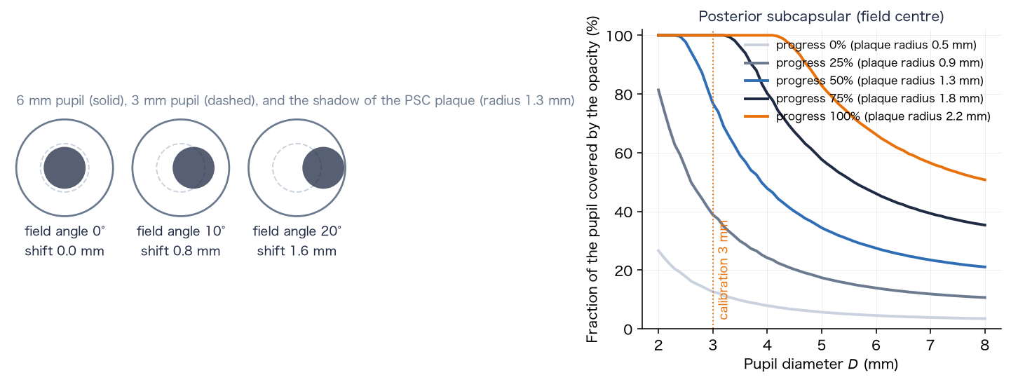
The covered fraction used for the scatter calculation is that of the field center only (the scatter is spread over the whole image with one kernel). How the plaque appears at the edge of the field is included in the core PSF of §7.
Key point: The increase in scatter due to an opacity becomes larger as the pupil becomes smaller (as the opacity covers more of the pupil), and is determined by the covered fraction at the center of the field.
9. Applying the PSF to the image (convolution)
This section shows how the PSF is applied to the image to calculate the terms of Eq. (7).
9-1. Convolution of the core
The core PSF is held as the coefficients of a grid (). The spacing of the grid (the texel pitch) is times the pixel, and the image is read from the mipmap level and convolved.
is the coefficient blended from the four nodes by Eq. (40), multiplied by the conservation coefficient .
9-2. Approximating the wide scatter with mipmaps
The wide scatter approximates the distribution determined by the CIE equation by a superposition of the mipmap levels of the image (each level half the size of the previous one). With the mean image of level , the scatter term is
is the mean of the center point and four points with rotated direction (radius ) at the pixel width ( pixels) of level (to avoid a square halo). The weights are decided by minimizing the sum of squared relative errors, so that the superposition of the kernels of the levels best fits the target distribution (radius pixels, pixel angle ; the argument of in degrees, in rad²).
The kernel of a level is the kernel that actually results when the mip of level is averaged at the five points above (computed numerically from the mip reduction and the five-point mean). The weights are fitted to the target distribution with this kernel. The upper limit of the scatter fraction is .
9-3. Combining into cone signals
The terms of Eq. (7) are calculated in the linear RGB of the capture space, converted to cone signals with the input matrix (Eq. (50)), and the lens with color adaptation (Eq. (22)) and the brightness correction (Eq. (24)) are reflected.
is the weight of the scatter increment over the reference eye, decided from of the chosen eye (Eq. (32)), and is the weight of the scatter of the reference eye (viewer's age ). is the component above white ( per channel; just before Eq. (7)). becomes linear display RGB through the tone mapping of §10.
Key point: The application to the image converts the sum of three terms (the convolution of the core, the mipmap approximation of the wide scatter, and the scatter of light above white) to cone signals and multiplies them by the cone-wise ratio of transmittances and the brightness correction.
10. Color calculation (cone space and Oklab)
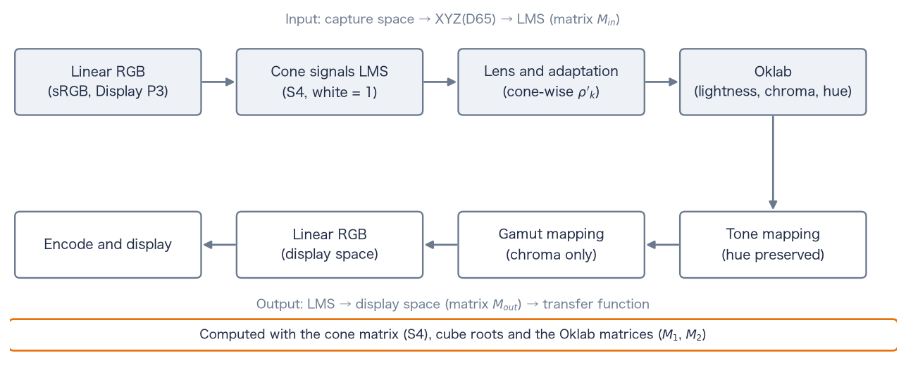
This section defines the color calculation of the app in cone space (LMS) and Oklab. The colors of the image are converted from linear RGB to cone signals, the lens (§4) is reflected, tone mapping is done in Oklab with the hue kept, and the result is returned to the display color space (Figure 12).
10-1. Color spaces and the cone matrix
The matrix from linear RGB to XYZ(D65) is derived from the chromaticities of the primaries and the chromaticity of the white point D65, . Let be the matrix whose columns are the direction vectors of the primaries, and the vector of the same form for the white point.
The chromaticities of the primaries are R, G, B for sRGB, and R, G, B for Display P3. The second row of this matrix is the contribution of each primary to luminance ( for sRGB; for Display P3).
The cone signals LMS are obtained by applying the cone matrix (cone system S4, a matrix that keeps the shape of the Hunt–Pointer–Estévez cones and is fitted to CIE 1964 10° XYZ [41]; normalized so that D65 white becomes ) to XYZ. The input matrix from the capture color space to LMS and the output matrix from LMS to the display color space are
For sRGB and S4 they are
10-2. Oklab
Oklab (Ottosson, 2020 [38]) is a uniform color space that forms lightness and two color axes from the cube roots of cone-like signals (LMS′). The app forms Oklab directly from the LMS of the chosen cone system.
and are Ottosson's matrices. The cube root keeps the sign ( for negative values). Hue is and chroma is . For achromatic colors and the lightness is the cube root of luminance (). Scaling LMS uniformly by scales by , so chromaticity and hue do not change.
10-3. Tone mapping
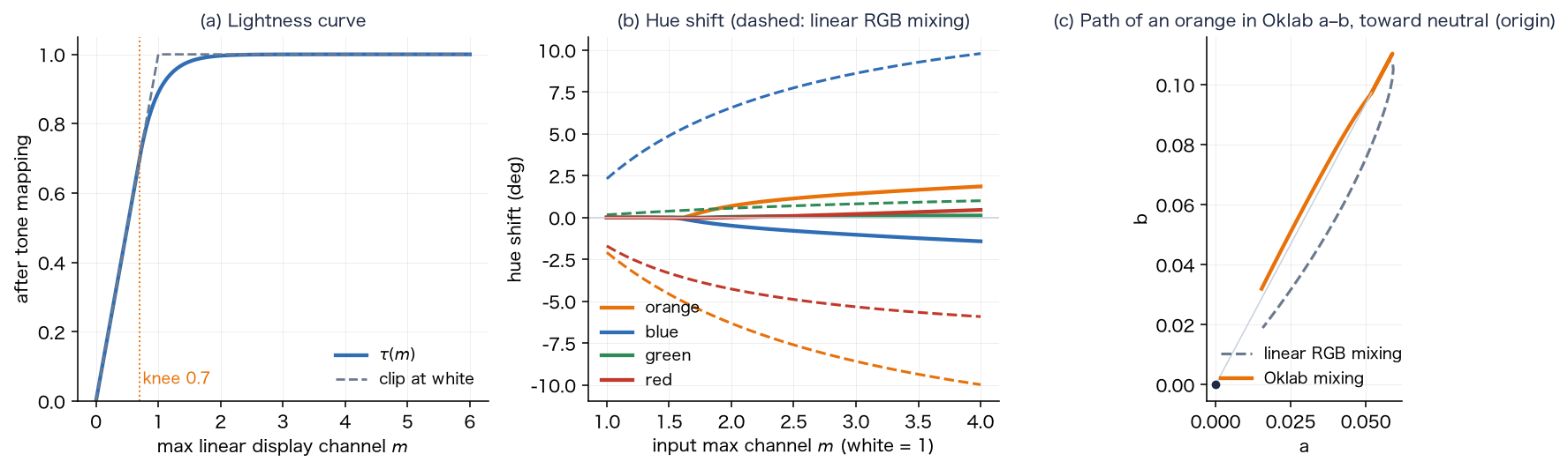
To fit the light of the screen into , the conversion uses the largest channel of the linear display RGB, , in three steps ( is computed from after step 1). Components below the knee are unchanged, but SDR white is above the knee and becomes .
- 1. Correction below the gamut: if reflecting the lens produces negative components in (outside the gamut), the Oklab lightness and hue are kept and only chroma is lowered, with the largest factor that removes the negative components (bisection).
- 2. Uniform scaling: a curve with a shoulder at the knee is applied to the largest channel, and the whole LMS is scaled uniformly (chromaticity and hue unchanged).
- 3. Path to white: only the component above the knee is moved toward the achromatic color of the same largest channel. This mixing is done in Oklab by reducing by a constant proportion, so the hue is kept.
in Eq. (55) are the values after the scaling of step 2. is the lightness of the achromatic color with the same largest channel. is returned to LMS by the inverse of Eq. (52), converted to linear display RGB with , and limited to .
10-4. Color spaces (sRGB and Display P3)
sRGB and Display P3 have the same transfer function (Eqs. (8), (9)) and differ only in their primaries. Only the primaries in Eqs. (49) and (50) are exchanged; the subsequent equations are the same. The capture color space is the color space in which the calculation receives the image. On the web, the browser converts the image to the display color space before passing it, so the capture space is Display P3 when the display is Display P3, and sRGB otherwise. The display color space follows the capability of the screen. The gain map is applied in the linear RGB of the capture space (Eq. (12)). The component above white is judged per channel of the linear RGB of the capture space (an approximation when the capture and display spaces differ).
Key point: The color calculation converts to LMS with the input matrix, reflects the lens and color adaptation cone by cone, tone-maps in Oklab with the hue kept, and returns to the display with the output matrix. sRGB and Display P3 use the same equations with exchanged primaries.
11. Progress and correspondence with clinical values
This section maps the progress of cataract to the scatter multiplier and to each parameter, and compares it with clinical values.
A progress takes the rows of the stage table (early, moderate, advanced) as the values at , and , and interpolates linearly between them. With the values of the stages , , ,
A progress of means the "early" values, not the absence of a contribution (a type contributes nothing only when it is not included). The increase in the scatter multiplier (added to normal ) is as follows.
| Type | Early (0%) | Moderate (50%) | Advanced (100%) |
|---|---|---|---|
| Nuclear | |||
| Cortical | (same as nuclear) | ||
| Posterior subcapsular | (1.82 times the nuclear multiplier) |
of a 65-year-old eye at the reference pupil (§8) is as follows.
| Type | 0% | 25% | 50% | 75% | 100% |
|---|---|---|---|---|---|
| Nuclear, cortical | 1.36 | 1.46 | 1.54 | 1.68 | 1.79 |
| Posterior subcapsular | 1.62 | 1.72 | 1.80 | 1.94 | 2.05 |
The moderate nuclear stage () was set close to the preoperative mean (§6-4). Cortical was made the same as nuclear because the increments over the normal values for the ages of the groups are small for both, nuclear and cortical (an assumption of this app). For posterior subcapsular, the mean is about higher than nuclear ( when the ages are matched), so the multiplier was set to times.
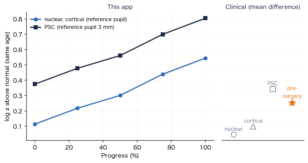
The comparison with clinical values is made not with absolute values but with increments. The groups of Gholami et al. differ in mean age (control 57, nuclear 63, cortical 62, posterior subcapsular 60 years), so the difference from the value of the age formula (33) at the mean age of each group is taken: nuclear (), cortical (), posterior subcapsular (). The of "early" is larger than the nuclear mean and close to the cortical mean (the stage values are an assumption of this app). The preoperative mean is about of the value of the age formula at 72 years, close to the of "moderate".
The above is the value for the scatter multiplier only. Light blocked by cortical wedges and the posterior subcapsular plaque is added to the scatter as well (§7-5). Near above , extending the of Eq. (30) over to makes the fraction of light going to scatter large ( at , at , at and at ). So there is a range where the upper limit () clips the result.
Key point: Progress is given by linear interpolation of the stage table. The increments of the scatter multiplier are matched to the age-matched increments of the clinical means (nuclear , cortical , posterior subcapsular in ) and to the preoperative mean.
12. Age, and what is not included
There is one age, and the "normal eye of the chosen age" and the "cataract eye" use the same age. Age acts on (1) the yellowing of the lens (Eq. (15)), (2) light scatter (Eq. (29)), and (3) the pupil (Eq. (27)). It does not act on the "original image".
It is known that nuclear cataract causes a myopic shift of refraction (an increase in the refractive power of the lens). However, myopic shift is a blur that glasses can correct. This app deals with how cataract looks in the corrected state (yellowing, scatter and glare), so the general settings do not reflect myopic shift (defocus). The value of the myopic shift ( of Eq. (37)) can be entered in the research settings.
Key point: Age acts on yellowing, scatter and the pupil, and myopic shift is not included in the general settings.
13. Limits
- It cannot be used for diagnosis, treatment or visual acuity tests. It differs from the way an individual sees. If you are concerned about symptoms of the eye, consult an eye doctor.
- Many of the numbers are guides (the table of §14 shows the values without a source).
- The brightness and color of the screen look different on different screens. The light source of an HDR scene cannot be reproduced on the screen (§2-5 reproduces it by supplementing scattered light).
- The assumption that the viewer's eye is equivalent to 20 years (§2). If the viewer is elderly, the "original image" also looks a little soft.
- It has no outputs such as visual acuity, contrast sensitivity or visual field.
- The knee of the tone mapping () also acts on SDR images; white becomes (§10-3).
- The age change of lens density uses the first-order equation of CIE 170-1, which differs in form from a report that it is linear on a squared age scale [6].
- The comparison with clinical values () was made with increments of means. The values of an individual eye can differ greatly from the mean (the standard deviation is to ).
Key point: This app is a tool for experiencing how things look, and many of its numbers are guides.
14. Parameter table and sources
For the 62 parameters and internal constants of this app, the value, source and level of confirmation are given. The names of the items are the names used in the research settings. The levels are as follows.
- A: checked by reading the original text (table, equation, section)
- B: only an abstract or summary was read
- C: checked in a secondary source (review, textbook, citation in another paper)
- D: no literature found (an assumption of this app; the reason is given in the remarks)
By level: A 5, B 1, C 20, D (no literature) 35, and 1 inputs and similar items. For items at level D, the reason for the choice is given in one line in the remarks. For the eye dimensions (Figure 2), the full texts of the main sources (Atchison et al. 2008, Strenk et al. 1999, Dubbelman and van der Heijde 2001, Navarro et al. 1985) could not be read, and the values are at level C.
14-1. Eye and scene
| Item | Symbol, default, unit, range | Sources | Level | Remarks |
|---|---|---|---|---|
| Age | , 65, years, 10–95 | — | — | An input. How age acts follows the source of each equation (§4 to §6). |
| Viewer age | , 20, years, 20–90 | — | D | No literature (an assumption of this app). Reason: a design choice to treat the eye that views the screen as a young normal eye (the reference eye) (§2). |
| Apply only the difference from a 20-year-old eye | 1 (general) / 0 (full eye model) | — | D | A design choice (§2), not a literature value. |
| Horizontal field of view | FOV, 50, deg, 10–120 | — | D | No literature (an assumption of this app). Reason: an input that depends on viewing conditions; it sets the field area of the pupil equation and the pixel angle. was taken as a typical apparent size. |
| White luminance of the image | , 200, cd/m², 1–3000. Night samples with street lighting use (Eq. (14)): cobblestone 13.13, plaza 17.5, night city 17.5, alley 7, park 5.25, snowy night 4.2. Other samples: indoors 100–250, daytime outdoors 3000–5000, paper 80 | [47][48][49] | C | Night scenes: the average road illuminance is from the P classes of EN 13201-2:2015 (P2 10, P3 7.5, P4 5, P5 3 lx; aligned with the classes of CIE 115:2010), and the road luminance uses cd/m²/lx of the road surface R3 of CIE 144:2001. The texts of the standards have not been read; the values are from secondary sources. The choice of class per scene and matching the image median to the road surface are assumptions of this app. Other scenes are estimates (paper as a perfect diffuser at 250 lx and reflectance 0.8 to 1.0 gives 64 to 80 cd/m², calculation ). The spread of haze is set by the ratio of lamp to road; the absolute level acts only on the pupil diameter and the degree of adaptation (§3-3). |
| Pupil diameter (0 = from brightness) | , 0 (automatic), mm, 0–8 | [1] | A | Equations 10, 17 and 21 of Watson and Yellott. The constants 846, 0.41, 7.75, 5.75, 28.58, 0.02132 and 0.009562 are those of the equations. The age term is based on data for 20 to 83 years; other ages (10 to 19, 84 to 95 years) are extrapolated. |
| Range of the pupil diameter | 2 to 8 mm | [33] | C | The textbook gives a pupil diameter of 2 to 8 mm. |
| Dark-adapted pupil | 7 mm (fixed) | [32] | D | No literature (an assumption of this app). Reason: a commonly used size for the dark-adapted pupil of young adults. That the pupil shrinks with age is suggested by the light-adapted result of [32], but no dark-adapted value was obtained. |
| Time constant of the pupil | 0.8 s (for constriction and dilation) | — | D | No literature (an assumption of this app). Reason: a value that avoids sudden changes of pupil diameter and flicker in camera video. |
| Degree of adaptation of L and M cones | , , (0.89 at cd/m²) | [44][39] | C | The CIECAM02 degree-of-adaptation equation (Eq. (23)). The original CIE 159 was not read. The equation was checked by our calculation to agree with the example in the colour-science documentation (). is the usual CIECAM02 choice of 20% of white as the adapting field. |
| Degree of adaptation of S cones | , 0.5, —, 0–1 (von Kries type, Eq. (22)) | [4][7] | D | No literature (an assumption of this app). Reason: the literature says only qualitatively that compensation along the yellow direction is incomplete, with no proportion [4][7]. was taken as a value smaller than that of the L and M cones. 0 means no adaptation; 1 returns white to achromatic. |
| Exponent of adaptation to brightness | , 0.5, —, 0–1 | — | D | No literature (an assumption of this app). Reason: set midway between full compensation (1) and none (0) for the adaptation to the drop in retinal illuminance caused by lens absorption. |
| Field-dependent opacity shadows | 1 (on) / 0 | — | D | A design choice (whether to include the parallax due to the depth of opacities; Eq. (39)). |
| Representative wavelengths of R, G and B for the PSF | 610, 550, 465 nm | — | C | Color is handled as cone signals; these three wavelengths are used only for the point spread function. The dominant wavelengths of the sRGB primaries (2° observer, D65), calculated, are R 611.4, G 549.1 and B 464.2 nm, differing by at most 1.4 nm (chromaticities of the primaries from a secondary source). The representative wavelengths are approximate. |
14-2. Nuclear (yellowing, myopic shift)
| Item | Symbol, default, unit, range | Sources | Level | Remarks |
|---|---|---|---|---|
| Lens optical density (spectral, age) | ; , ; 0.20 at 20 and 0.49 at 65 years (450 nm) | [35][12][6] | C | The table of the two components and is that of CIE 170-1 (distributed with the model of Asano et al.; agrees with the 32-year table of Stockman, Sharpe and Fach at 400 nm and above). The age factor is the CIE 170-1 equation, checked in the text of Asano et al. (the CIE document itself has not been read). The age change at 400 nm is 0.13 per decade up to 60 years and 0.44 above, close to the 0.12 and 0.40 of the abstract of Pokorny et al. [12]. A report describes the age change as linear on a squared age scale [6], but the first-order equation of CIE 170-1 is used. |
| Increment of optical density for nuclear cataract | , +0.07 / +0.13 / +0.26 (early / moderate / advanced), OD; spectral shape (same as the age-dependent component) | [4][12][25][26] | C | Spectral shape: Delahunt et al. fitted the density of cataractous lenses with the spectral shape of the aging component (the of Pokorny et al.) [4]. Nuclear cataract has no new absorption band [25][26]. Magnitude: Delahunt et al. report that lenses with grade 2–3+ cataract reduced light by about 40% [4]. The value that gives 60% luminance transmittance at age 70 is (calculation in this paper), so the moderate stage is 0.13. The early and advanced stages (about 1/2 and 2 times the moderate stage) are assumptions of this app. |
| Myopic shift (defocus) | , 0 (general), D, −4–8. The stage table gives 0.5 / 1.5 / 3.0 D | [24] | D | No literature for the magnitude. The spherical-equivalent change of the nuclear cataract group is −0.38 (0.60) D [24]. Reason: the general settings deal with the corrected state and do not reflect it (§12). The stage values for research were set as guides that grow with nuclear sclerosis. |
| Chromatic aberration | (D, in nm) | [18][36] | C | Agrees with the coefficients and of the Thibos equation ([36] full text). The reference wavelength is 550 nm, and only differences are used. |
| Spherical aberration (Z4,0 RMS, 6 mm pupil) | , −0.10 / −0.25 / −0.45 µm (early / moderate / advanced), µm, −1–1 | [22][23] | D | No literature for the stage values (an assumption of this app). The sign agrees with the literature (negative in nuclear cataract) [22][23]. Magnitude: −0.35 ± 0.41 µm for the nuclear group in internal optics at 6 mm [23]. 0.10 to 0.45 µm is within that range, but the correspondence to the stages is not in the literature (an assumption of this app). |
14-3. Cortical (spokes)
| Item | Symbol, default, unit, range | Sources | Level | Remarks |
|---|---|---|---|---|
| Number of spokes | 12 (3–24) | [15][20] | D | No literature (an assumption of this app). Reason: cortical opacities appear as spokes [15], and the Wisconsin grading assesses cortical opacity by sectors of the periphery [20]; the number represents many spokes arranged around the periphery. |
| Spoke extent toward the center | 0.25 / 0.6 / 0.95 (early / moderate / advanced), 0–1 | [21] | D | No literature (an assumption of this app). Reason: clinical scales use area fractions and do not define the length of a spoke. A trial conversion of the spoke area to the AREDS scale (calculation in this paper) gives 7 / 29 / 65% of the whole lens and 0 / 21 / 65% of the central 5 mm circle. |
| Angular occupancy of spokes | 0.15 / 0.35 / 0.65, 0–1 | [21] | D | No literature (an assumption of this app). Reason: as above. AREDS uses a continuous area %; no discrete early, moderate or advanced classes are defined. |
| Spoke opacity (fraction of light blocked) | , 0.3 / 0.5 / 0.75, 0–1 | — | D | No literature (an assumption of this app). Reason: no report measuring the transmission of a spoke was found. The total scatter was calibrated to the C-Quant (§6, §11). |
| Spoke roughness (OPD RMS) | , 0.5 / 0.9 / 1.3 µm, 0–3 | — | D | No literature (an assumption of this app). Reason: no report measuring the phase disturbance inside an opacity was found. Set as a magnitude that gives a scatter-like disturbance to the PSF. |
| Radius where the spokes begin | 4 mm (the outer 1 mm of the 5 mm lens radius) | [15] | D | No literature (an assumption of this app). Reason: cortical opacity is represented as spokes extending from the periphery toward the center (the form of this app); 4 mm was set as the outer 1 mm of the lens. |
14-4. Opacity placement and depth
| Item | Symbol, default, unit, range | Sources | Level | Remarks |
|---|---|---|---|---|
| Spoke depth behind the pupil plane | , 0.8, mm, 0–6 | [21][15] | D | No literature (an assumption of this app). Reason: cortical opacities occur in both the anterior and posterior cortex [21]. The anterior cortex was taken as representative and placed near the pupil plane. |
| Spoke direction, angular width of the sector | 180° (left), 360° (all around) | — | D | A definition (the setting of the sector in which spokes are placed), not a literature value. |
| Plaque depth behind the pupil plane | , 4.5, mm, 0–8 | [15][14][13] | C | A posterior subcapsular opacity forms at the posterior pole in front of the posterior capsule [15]. The distance from the pupil plane to the pole equals the lens thickness: 4 mm in a model eye [13], and 3.60 mm at 20, about 4.5 mm at 50 to 60 and 4.77 mm at 70 years by the age equation [14]. |
| Plaque center offset, aspect ratio, long-axis angle | 0 mm (horizontal, vertical), 1 (circle), 0° | — | D | Definitions (settings of the position and shape of the plaque), not literature values. |
14-5. Posterior subcapsular (central plaque)
| Item | Symbol, default, unit, range | Sources | Level | Remarks |
|---|---|---|---|---|
| Central plaque radius | 0.5 / 1.3 / 2.2 mm (early / moderate / advanced), 0–4 | [21][19] | D | No literature (no clinical size in mm was found). A trial conversion to the AREDS scale (% of the area of the central 5 mm circle; calculation in this paper) gives 4 / 27 / 77%. The AREDS example is 15% and the case threshold is 5%. |
| Plaque opacity (fraction of light blocked) | , 0.3 / 0.55 / 0.8, 0–1 | [3] | D | No literature (an assumption of this app). Reason: no measurement of the transmission of a plaque was found. Set larger than for nuclear, in line with the highest (1.48) of posterior subcapsular cataract [3]. |
| Plaque roughness (OPD RMS) | , 0.6 / 1.0 / 1.4 µm, 0–3 | — | D | No literature (an assumption of this app). Reason: as for the spoke roughness (above). |
14-6. Straylight
| Item | Symbol, default, unit, range | Sources | Level | Remarks |
|---|---|---|---|---|
| Straylight multiplier (normal eye = 1) | , 1, ×, 1–30 | [2][34] | B | The CIE age-corrected Stiles–Holladay equation (valid from 1° to 30°). The constants 10, 70 and 4 were confirmed in the abstract [34]. The CIE document itself was not read. |
| Straylight increment for cataract | nuclear, cortical +0.3 / +1.0 / +2.5; posterior subcapsular +1.37 / +2.64 / +5.37 (1.82 times the nuclear multiplier) | [3][5] | C | Matched to the clinical increments in (over the normal value at the mean age of each group: nuclear +0.05, cortical +0.10, posterior subcapsular +0.34; the preoperative mean is about ×1.8 of the age equation) (§11). The values per stage are a design of this app. |
| PSC and cortical straylight increments | values of the table above (for the reference coverage; scaled by the covered fraction) | — | D | That the increment is proportional to the covered fraction is an assumption from physics; support from measurement is unconfirmed (§8). |
| Reference pupil for the straylight increment | 3 mm for PSC, 6 mm for cortical | [31] | D | No literature (an assumption of this app). Reason: the pupil size of clinical measurements could not be confirmed in each paper. For PSC, a value close to clinical conditions; for cortical, 6 mm because at some stages the spokes do not reach a 3 mm pupil. For natural pupils (2 to 7 mm), straylight hardly depends on pupil size [31]. |
| Angular distribution (constant inside 1°, outside 30°) | , | [2][34] | D | The range of validity (1° to 30°) is from [34]. The joining outside the range is not in the literature (an assumption of this app). Reason: to give a finite scatter up to the edge of the image, it was joined continuously. |
14-7. Internal constants and numerical settings
| Item | Symbol, default, unit, range | Sources | Level | Remarks |
|---|---|---|---|---|
| Destination of blocked light | scatter 80%, absorption 20%, upper limit of the scatter fraction 90% | [27] | D | No literature (no study measuring the split between absorption and scatter was found). Mie calculations predict that 99.8% of incident light is scattered for one Indian nuclear cataract, and less than 20% for immature US cataracts [27]; the scatter is strongly forward, unlike wide scatter. Reason: to treat most of the light loss of an opacity as scatter. |
| Stiles–Crawford effect | , 0.05, mm⁻² (intensity ) | [30][33] | C | Within the literature range: 0.047 ± 0.013 (670 nm), 0.0636 (550 nm) [30], textbook value 0.066 [33]. |
| Lens radius | 5 mm | [14] | D | Equatorial diameters of in vivo MRI are reported at about 8.4 to 9 mm (radius 4.2 to 4.5 mm), so 5 mm is on the large side (secondary source). Reason: set generously as the upper bound for the placement of spokes and plaques. |
| Correlation length of roughness, width of the plaque edge | 0.3 mm, 0.3 mm | — | D | No literature (an assumption of this app). Reason: set as the smallest smoothness that the numerical grid of the pupil plane (0.04 mm or finer) can represent. |
| Distance of the cone of light | , 20.4, mm (pupil plane to retina) | [13] | C | The axial length of about 24 mm minus about 3.6 mm for the cornea and chamber (model eye [13], age equation [14]). |
| Field nodes, core grid | 3×3 nodes, grid () | — | D | Numerical settings, not literature values. Chosen as a balance between accuracy and cost. |
14-8. Image, HDR and display
| Item | Symbol, default, unit, range | Sources | Level | Remarks |
|---|---|---|---|---|
| Cone system (LMS) | S4 (HPE shape, 10°); D65 white = (1,1,1) | [41][40] | C | The spectral sensitivities are obtained by applying this matrix to the CIE 1964 10° color-matching functions (Eq. (20)). |
| Weighting light for the cone-wise transmittance | standard illuminant D65, 380–780 nm at 5 nm | [42] | A | Chosen because the display white is equivalent to D65. Exact for narrow-band light, approximate for broad-band light (§4-2). |
| Oklab matrices | , (Ottosson) | [38] | C | for the chosen cone system. |
| Primaries of the color spaces | sRGB, Display P3 (white point D65) | [10][43] | C | On the web, the capture space is the display space into which the browser converts the image (P3 when the display is P3). |
| Correction below the gamut | bisection, 24 iterations (16 in the shader; chroma only) | — | D | A numerical setting (Eq. (53)). Only chroma is changed, to keep lightness and hue. |
| sRGB transfer function | 12.92, 0.055, 2.4, 0.04045, 0.0031308 | [16][10] | A | Item 8 of [16] was read (the standard itself [10] was not read). |
| Luminance coefficients | 0.2126, 0.7152, 0.0722 | [17] | A | Item 3.2 of ITU-R BT.709-6 was read. |
| Gain map equations | , | [8][9] | A | Equivalent to the equation of the Android specification (weight ). The text of ISO 21496-1 was not read. |
| Gain map offset (samples) | , 1/512 | [8] | D | No literature (a choice of this app). The default of the Android specification is 1/64 (0.015625). Reason: a small value was chosen to reduce errors in the dark parts of the samples. For a photo with a gain map, the values in the file are used. |
| Upper limit of the gain | — | D | An implementation limit (to fit the maximum 65504 of half-precision floating point). The shader that applies the gain map limits to this value. | |
| Knee and white path of the tone mapping | , white-path width 4 (mixed in Oklab) | [29][38] | D | No literature (own design). Reason: there is no standard curve for display of photographs and the web (BT.2408 is guidance for video). Below the knee the curve is linear, and bright components above the knee are rounded (SDR white 1.0 also becomes 0.889). The path to white is done in Oklab, reducing the hue shift from about 10° with linear mixing in RGB to within 2° (Figure 11). |
| Headlight intensity and distance (synthetic sample) | 800 cd (per lamp), about 32 m | [28] | D | The upper limit of a passing beam toward the oncoming driver (B50L) in UN R112 is 350 cd, and 1,750 cd at BR. 800 cd exceeds the B50L limit and is below the BR limit. Reason: an assumption to reproduce the strong glare of a headlight. |
| Clipping of HDRIs and lowering of white luminance | 300 times the median, cd/m², scene maximum cd/m² | — | D | No literature (an assumption of this app). Reason: to suppress the unrealistic values of three original HDRIs in which the exit, sky or light source is orders of magnitude brighter than reality. |
14-9. Eye dimensions (Figure 2)
| Item | Symbol, default, unit, range | Sources | Level | Remarks |
|---|---|---|---|---|
| Axial length | about 24 mm (corneal apex to inner retinal surface) | [13][14] | C | 24.197 mm in the model eye (sum) [13]. By the in vivo age equation, 23.21 mm at 20 and 23.78 mm at 70 years [14]. |
| Cornea and anterior chamber | about 3.6 mm (cornea 0.55, chamber about 3.05) | [13][14] | C | 0.55 + 3.05 in the model eye [13]. The chamber becomes shallower with age (3.11 mm at 20 and 2.58 mm at 70 years by the age equation) [14]. |
| Lens thickness | about 4.5 mm (Figure 2; guide for 50 to 60 years) | [13][14] | C | 4 mm in the model eye [13]; 3.60 mm at 20 and 4.77 mm at 70 years by the age equation [14]. |
| Vitreous cavity | about 16 mm | [13] | C | 16.597 mm in the model eye [13]. About 16 mm or slightly less in young adults in vivo. |
| Retina, macula and optic disc | retinal thickness about 0.25 mm, fovea about 1.5 mm, disc about 1.9 × 1.8 mm, fovea about 3.4 mm temporal to the disc margin | [37] | C | Secondary citation (values of Polyak 1941 and others). |
| Entrance pupil magnification | about 1.13 (the pupil of Figure 2 is the actual iris aperture) | [33] | C | The textbook states that the cornea magnifies the iris image by a factor of 1.13. The pupil diameter of the Watson and Yellott equation corresponds to the entrance pupil. |
Key point: The values are distinguished into those confirmed in the literature (levels A and B), those confirmed in secondary sources (C), and assumptions without literature (D). For items at level D the reason for the choice is given in the remarks.
References
[1] A. B. Watson and J. I. Yellott, "A unified formula for light-adapted pupil size", Journal of Vision, vol. 12, no. 10, article 12, 2012. doi:10.1167/12.10.12 — Checked: Equations 10, 17 and 21 were checked in the full text.
[2] CIE 146:2002, CIE Equations for Disability Glare, in CIE Collection on Glare 2002 (CIE 146/147:2002), Commission Internationale de l'Éclairage (including the age-dependent Stiles–Holladay equation); see also CIE 135/1:1999, Disability glare, J. J. Vos — Checked: The scope was checked on the CIE page, and the form of the equation in the abstract of [34]. The CIE document itself has not been read.
[3] S. Gholami, N. J. Reus, and T. J. T. P. van den Berg, "Changes in intraocular straylight and visual acuity with age in cataracts of different morphologies", Journal of Ophthalmology, vol. 2017, article 5649532, 2017, Table 4 and Equation 1. doi:10.1155/2017/5649532. https://pmc.ncbi.nlm.nih.gov/articles/PMC5554999 — Checked: Table 4 and Equation 1 were checked in the full text (the equation in MathML).
[4] J. Delahunt, M. A. Webster, L. Ma, and J. S. Werner, "Long-term renormalization of chromatic mechanisms following cataract surgery", Visual Neuroscience, vol. 21, 2004. https://pmc.ncbi.nlm.nih.gov/articles/PMC2633455 — Checked: Read in full. The proportion of compensation is not given.
[5] I. J. E. van der Meulen, J. Gjertsen, B. Kruijt, J. P. Witmer, A. Rulo, R. O. Schlingemann, and T. J. T. P. van den Berg, "Straylight measurements as an indication for cataract surgery", Journal of Cataract & Refractive Surgery, vol. 38, no. 5, pp. 840–848, 2012. doi:10.1016/j.jcrs.2011.11.048 — Checked: The values (1.55, 1.29) were checked in the abstract. The full text has not been obtained.
[6] R. van de Kraats and D. van Norren, "Optical density of the aging human ocular media in the visible and the UV", Journal of the Optical Society of America A, vol. 24, no. 7, pp. 1842–1857, 2007. doi:10.1364/josaa.24.001842 — Checked: Abstract only. The age change is described as linear in a squared age scale, a form different from the app's equation (first order in age).
[7] J. M. Kraft and J. S. Werner, "Aging and the saturation of colors. 2. Scaling of color appearance", Journal of the Optical Society of America A, vol. 16, no. 2, pp. 231–235, 1999. doi:10.1364/josaa.16.000231 — Checked: Abstract only: substantial compensation over a range of densities, incomplete at the highest density.
[8] Android Developers, "Ultra HDR image format", version 1.1. https://developer.android.com/media/platform/hdr-image-format — Checked: Read in full (the equation of the Display section, the HDR Gain map metadata table, the note in Gain map generation).
[9] ISO 21496-1:2025, Digital photography — Gain map metadata for image conversion — Part 1: Dynamic range conversion, International Organization for Standardization, 2025 — Checked: Only the title and its treatment in the Android specification were checked. The text has not been read.
[10] IEC 61966-2-1:1999, Multimedia systems and equipment — Colour measurement and management — Part 2-1: Colour management — Default RGB colour space — sRGB, and Amendment 1:2003, International Electrotechnical Commission — Checked: The standard itself has not been read. The constants were checked in the explanation [16].
[11] Sample images: HDRIs (CC0) from Poly Haven (https://polyhaven.com/license) and ambientCG (https://docs.ambientcg.com/license/).
[12] J. Pokorny, V. C. Smith, and M. Lutze, "Aging of the human lens", Applied Optics, vol. 26, no. 8, pp. 1437–1440, 1987. doi:10.1364/ao.26.001437 — Checked: Abstract only (density at 400 nm: 0.12 per decade from 20 to 60 years, 0.40 per decade above 60). The tables and equations were not read.
[13] Gullstrand–Le Grand schematic eye (relaxed), as tabulated in the lecture notes of the Visual Optics Lab, University of Arizona, "Class02_08". https://wp.optics.arizona.edu/visualopticslab/wp-content/uploads/sites/52/2016/08/Class02_08.pdf — Checked: The table (cornea 0.55, chamber 3.05, lens 4, vitreous 16.597 mm) was read. The original Gullstrand and Le Grand sources have not been read.
[14] S. Giovanzana, T. Evans, and B. Pierscionek, "Lens internal curvature effects on age-related eye model and lens paradox", Biomedical Optics Express, vol. 8, no. 11, pp. 4827–4837, 2017, Table 1. doi:10.1364/BOE.8.004827. https://pmc.ncbi.nlm.nih.gov/articles/PMC5695934 — Checked: The age equations of Table 1 were read.
[15] Webvision, "Crystalline lens and cataract". https://www.webvision.pitt.edu/?p=7859 — Checked: Read in full (positions of the types; cortex and nucleus cannot be separated histologically; the posterior subcapsular opacity is at the posterior pole in front of the posterior capsule). Secondary source.
[16] International Color Consortium and W3C, "How to interpret the sRGB color space (specified in IEC 61966-2-1) for ICC profiles". https://www.w3.org/Graphics/Color/srgb — Checked: The transfer function of item 8 was read.
[17] ITU-R Recommendation BT.709-6, Parameter values for the HDTV standards for production and international programme exchange, 2015. https://www.itu.int/dms_pubrec/itu-r/rec/bt/R-REC-BT.709-6-201506-I!!PDF-E.pdf — Checked: The luminance equation of item 3.2 was read.
[18] L. N. Thibos, M. Ye, X. Zhang, and A. Bradley, "The chromatic eye: a new reduced-eye model of ocular chromatic aberration in humans", Applied Optics, vol. 31, no. 19, pp. 3594–3600, 1992. doi:10.1364/ao.31.003594 (coefficients as quoted in the text of [36]) — Checked: Only the abstract of Thibos et al. was read. The coefficients were checked in [36] (secondary).
[19] L. T. Chylack Jr. et al., "The Lens Opacities Classification System III", Archives of Ophthalmology, vol. 111, pp. 831–836, 1993. doi:10.1001/archopht.1993.01090060119035 — Checked: Abstract only (standard images: 6 each for NC and NO, 5 for cortical, 5 for posterior subcapsular; decimal scale). The definitions of area and size for cortical and posterior subcapsular grades could not be read.
[20] B. E. K. Klein, R. Klein, and K. E. Lee, "Incidence of age-related cataract: the Beaver Dam Eye Study", Archives of Ophthalmology, vol. 116, no. 2, pp. 219–225, 1998 — Checked: The abstract and bibliographic data were checked. The details of the grading could not be confirmed (the text was not read).
[21] AREDS Research Group, "The Age-Related Eye Disease Study system for classifying cataracts from photographs: AREDS report no. 4", American Journal of Ophthalmology, vol. 131, pp. 167–175, 2001. https://pmc.ncbi.nlm.nih.gov/articles/PMC2032014 — Checked: Read in full (cortical and posterior subcapsular opacities as a % of the area of the central 5 mm circle; a continuous scale; no discrete severity classes are defined).
[22] T. Kuroda, T. Fujikado, N. Maeda, T. Oshika, Y. Hirohara, and T. Mihashi, "Wavefront analysis in eyes with nuclear or cortical cataract", American Journal of Ophthalmology, vol. 134, pp. 1–9, 2002. doi:10.1016/s0002-9394(02)01402-2 — Checked: Abstract only. Spherical aberration is negative in nuclear and positive in cortical cataract (6 mm pupil). The magnitude (µm) is not in the abstract.
[23] Wu, Jin, Shen, Li, and Cui, "Wavefront aberrations and retinal image quality in different lenticular opacity types and densities", Scientific Reports, vol. 7, article 15247, 2017. doi:10.1038/s41598-017-15245-4. https://pmc.ncbi.nlm.nih.gov/articles/PMC5681554 — Checked: Table 2 was read (internal optics, 6 mm, spherical-like aberration: nuclear −0.35 ± 0.41 µm, cortical 0.08 ± 0.14, posterior subcapsular 0.11 ± 0.17).
[24] K. Pesudovs and D. B. Elliott, "Refractive error changes in cortical, nuclear, and posterior subcapsular cataracts", British Journal of Ophthalmology, vol. 87, pp. 964–967, 2003. doi:10.1136/bjo.87.8.964 — Checked: The abstract and bibliographic data were checked (spherical-equivalent change of the nuclear cataract group −0.38 (0.60) D). The full text could not be confirmed.
[25] J. Mellerio, "Yellowing of the human lens: nuclear and cortical contributions", Vision Research, vol. 27, pp. 1581–1587, 1987. doi:10.1016/0042-6989(87)90166-0 — Checked: Abstract only. In the nucleus the pigment increases; in the cortex the path length increases.
[26] S. Siik, L. T. Chylack, J. Friend, J. Wolfe, J. Teikari, H. Nieminen, and P. J. Airaksinen, "Lens autofluorescence and light scatter in relation to the lens opacities classification system, LOCS III", Acta Ophthalmologica Scandinavica, vol. 77, pp. 509–514, 1999. doi:10.1034/j.1600-0420.1999.770504.x — Checked: Abstract only. NC and the autofluorescence index r = −0.71; NO and light scatter r = 0.64.
[27] K. O. Gilliland, S. Johnsen, S. Metlapally, M. J. Costello et al., "Mie light scattering calculations for an Indian age-related nuclear cataract with a high density of multilamellar bodies", Molecular Vision, vol. 14, pp. 572–582, 2008. https://pmc.ncbi.nlm.nih.gov/articles/PMC2275208 — Checked: Read in full. Model predictions (not measurements): 99.8% of incident light at 550 nm scattered for one Indian nuclear cataract; less than 20% for immature US cataracts.
[28] UN Regulation No. 112, Uniform provisions concerning the approval of motor vehicle headlamps emitting an asymmetrical passing-beam or a driving-beam or both and equipped with filament lamps and/or light-emitting diode (LED) modules, 6.2.4. https://www.mlit.go.jp/jidosha/un/UN_R112.pdf — Checked: The light distribution table of 6.2.4 was read (maximum 350 cd at B50L, 1,750 cd at BR).
[29] ITU-R Report BT.2408-8, Guidance for operational practices in HDR television production, 2024 — Checked: Read. There is no standard curve for still pictures (Annex 5 has only a knee for PQ display). The later BT.2408-9 has not been read.
[30] R. A. Applegate and V. Lakshminarayanan, "Parametric representation of Stiles–Crawford functions: normal variation of peak location and directionality", Journal of the Optical Society of America A, vol. 10, no. 7, pp. 1611–1623, 1993. doi:10.1364/JOSAA.10.001611; and W. S. Stiles, Proceedings of the Royal Society B, vol. 123, pp. 90–118, 1937. — Checked: Checked through values cited in a secondary source (ρ = 0.047 ± 0.013 mm⁻² horizontally; Stiles 0.0636 mm⁻² at 550 nm). The originals have not been read.
[31] L. Franssen, J. Tabernero, J. E. Coppens, and T. J. T. P. van den Berg, "Pupil size and retinal straylight in the normal eye", Investigative Ophthalmology & Visual Science, vol. 48, no. 5, pp. 2375–2382, 2007 — Checked: Read in full. For natural pupils (2 to 7 mm), straylight hardly depends on pupil size (within 0.2 log units).
[32] B. Winn, D. Whitaker, D. B. Elliott, and N. J. Phillips, "Factors affecting light-adapted pupil size in normal human subjects", Investigative Ophthalmology & Visual Science, vol. 35, no. 3, pp. 1132–1137, 1994 — Checked: Abstract only. The light-adapted pupil diameter decreases linearly with age (not a dark-adapted value).
[33] H. Gross (ed.), Handbook of Optical Systems, vol. 4, chapter 36 "Human eye", Wiley-VCH, 2008, ISBN 978-3-527-40380-6 — Checked: The PDF text was read (pupil diameter 2 to 8 mm, entrance-pupil magnification 1.13, Stiles–Crawford p = 0.066). Textbook.
[34] J. J. Vos, "On the cause of disability glare and its dependence on glare angle, age and ocular pigmentation", Clinical and Experimental Optometry, vol. 86, no. 6, pp. 363–370, 2003. doi:10.1111/j.1444-0938.2003.tb03080.x — Checked: Abstract only. L_veil/E = 10(1 + (Age/70)⁴)/θ² (1° to 30°) was confirmed.
[35] Y. Asano, M. D. Fairchild, and L. Blondé, "Individual colorimetric observer model", PLoS ONE, vol. 11, no. 2, e0145671, 2016, Eqs. 2–4, citing CIE 170-1:2006. https://pmc.ncbi.nlm.nih.gov/articles/PMC4749337; the two-component ocular media density table of CIE 170-1 distributed with the model (as included in luxpy, https://github.com/ksmet1977/luxpy); and the lens density table of Stockman, Sharpe and Fach (1999), CVRL, http://www.cvrl.org/maclens.htm — Checked: Equations 2–4, the two-component table and the CVRL table were read (CIE 170-1 itself has not been read).
[36] D. H. Marimont and B. A. Wandell, "Matching color images: the effects of axial chromatic aberration", Journal of the Optical Society of America A, vol. 11, pp. 3113–3122, 1994 — Checked: Read in full (the coefficients 0.63346 and 0.21410 of the Thibos equation; 1.7312 is the value chosen by Marimont and Wandell for a 580 nm reference).
[37] Webvision, "Facts and figures concerning the human retina". https://www.webvision.pitt.edu/?p=35 — Checked: Read in full (retinal thickness, fovea 1.5 mm, optic disc 1.86 × 1.75 mm). No source is given for the optic disc values.
[38] B. Ottosson, "A perceptual color space for image processing", blog post, 23 December 2020. https://bottosson.github.io/posts/oklab/ — Checked: The values of the matrices M1 and M2 were used.
[39] M. D. Fairchild, Color Appearance Models, 3rd ed., John Wiley & Sons, 2013. doi:10.1002/9781118653128 — Checked: Cited for the form of von Kries-type adaptation. The text has not been read.
[40] JIS Z 8701:1999, Colour specification — The CIE 1931 standard colorimetric system and the CIE 1964 supplementary standard colorimetric system (in Japanese), Japanese Standards Association, Annex, Table 2 (CIE 1964 10° color-matching functions) — Checked: The values were transcribed from the appendix table of the JIS handbook.
[41] R. W. G. Hunt and M. R. Pointer, "A colour-appearance transform for the CIE 1931 standard colorimetric observer", Color Research & Application, vol. 10, no. 3, pp. 165–179, 1985. doi:10.1002/col.5080100306 — Checked: The basis of the cone system S4 (a matrix that keeps the shape of the HPE cones and is fitted to 10° XYZ). The text has not been read.
[42] CIE standard illuminant D65, table of the Colour & Vision Research Laboratory. http://www.cvrl.org/database/data/cie/Illuminantd65.csv — Checked: The table values were read and used at 5 nm.
[43] SMPTE EG 432-1:2010, Digital Source Processing — Color Processing for D-Cinema; and Apple Inc., "Display P3", ICC Registry. https://registry.color.org/rgb-registry/displayp3 — Checked: The chromaticities of the primaries were used. The texts have not been read.
[44] CIE 159:2004, A Colour Appearance Model for Colour Management Systems: CIECAM02; and N. Moroney, M. D. Fairchild, R. W. G. Hunt, C. Li, M. R. Luo, and T. Newman, "The CIECAM02 color appearance model", IS&T/SID Tenth Color Imaging Conference, pp. 23–27, 2002 — Checked: Neither text was read. The degree-of-adaptation equation was checked against the colour-science documentation (the example of colour.adaptation.degree_of_adaptation) and the Wikipedia article on CIECAM02.
[45] CIE 170-1:2006, Fundamental Chromaticity Diagram with Physiological Axes — Part 1, Commission Internationale de l'Éclairage, 2006 — Checked: The text has not been read. The equation and table of the two-component density were checked in [35].
[46] A. Stockman, L. T. Sharpe, and C. Fach, "The spectral sensitivity of the human short-wavelength sensitive cones derived from thresholds and color matches", Vision Research, vol. 39, no. 17, pp. 2901–2927, 1999. Lens density table: CVRL, http://www.cvrl.org/maclens.htm — Checked: The CVRL table (lensss_5) was read. The paper has not been read.
[47] CIE 115:2010, Lighting of Roads for Motor and Pedestrian Traffic, Commission Internationale de l'Éclairage, 2010 — Checked: The text has not been read. The correspondence of classes follows [48].
[48] EN 13201-2:2015, Road lighting — Part 2: Performance requirements, European Committee for Standardization, 2015, Table 3 (P classes) — Checked: The text has not been read. The average illuminances of the P classes (P2 10, P3 7.5, P4 5, P5 3 lx) are from secondary sources.
[49] CIE 144:2001, Road Surface and Road Marking Reflection Characteristics, Commission Internationale de l'Éclairage, 2001 — Checked: The text has not been read. The average luminance coefficient q0 = 0.07 cd/m²/lx of the standard road surface R3 is from secondary sources.