Brighter and Bigger

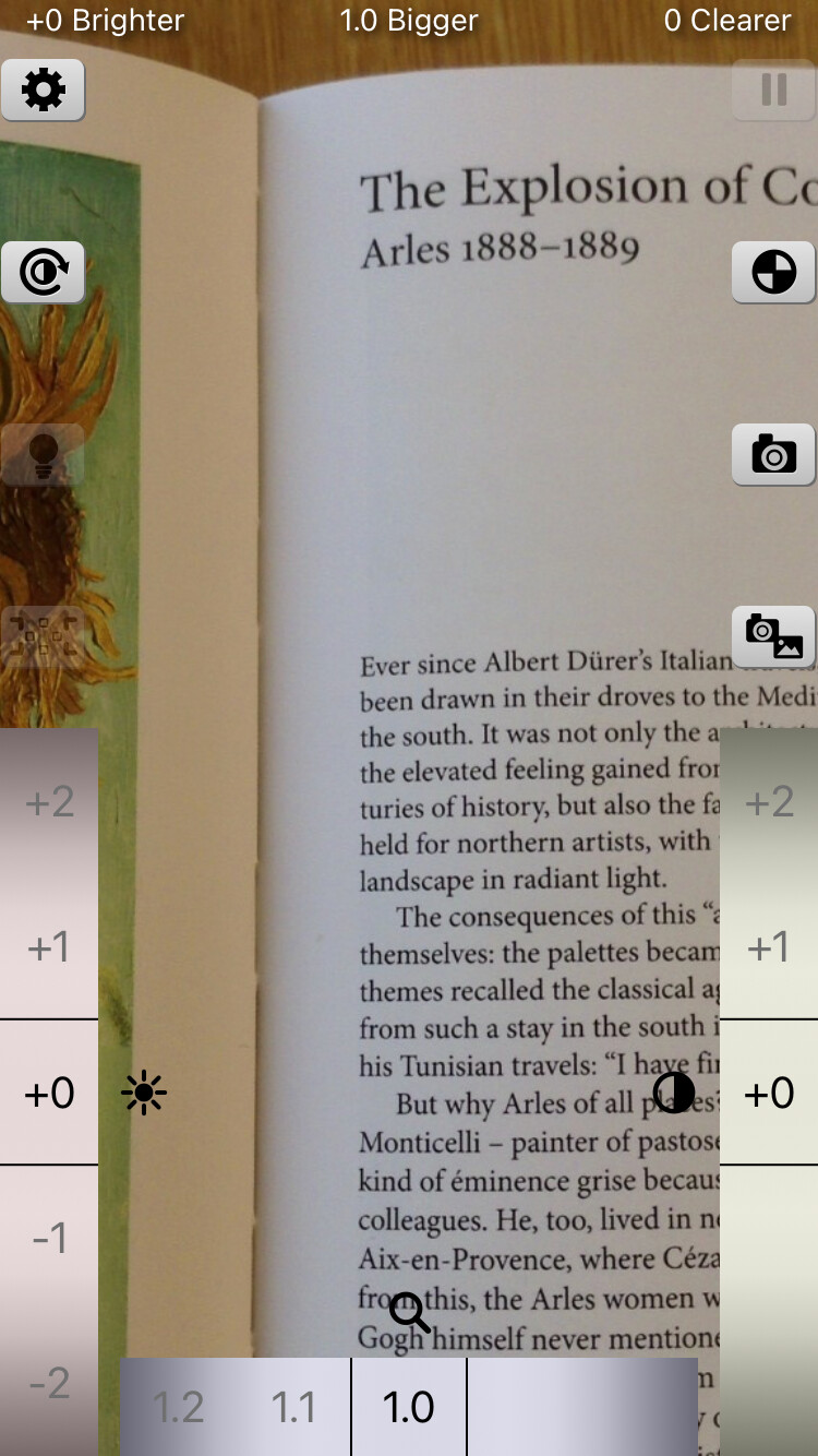
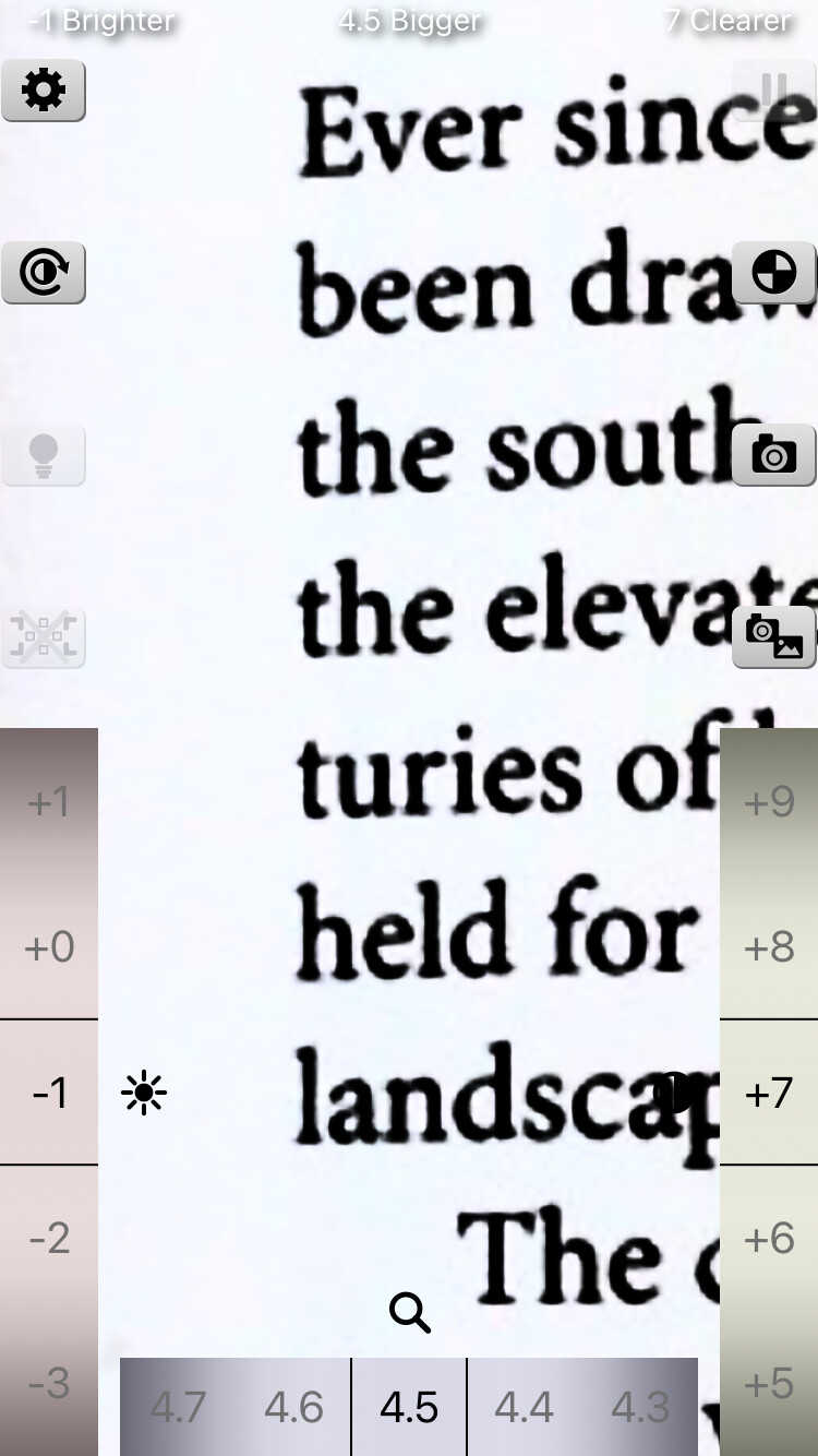
Theory of Brighter and Bigger 3.0

1. Overview

This paper describes the color transformation that the app "Brighter and Bigger" 3.0 applies to improve the legibility of an image. The framework of this paper is a reorganization, for version 3.0, of the mathematical expressions in the appendix of the README of version 2.0 of the same app [1]. The essential point is that only the lightness is changed while the chromaticity is preserved. Because only the lightness is manipulated, the hue does not change, and only the difference between light and dark is emphasized.

1-1. Assumptions

The following are assumed throughout this paper.

1. 1. White point: D65, $(x,y)=(0.3127,\,0.3290)$ (the defined value in the sRGB and Display P3 standards [2][3][4]). It is common to all conversions.

1. 2. Observer: the CIE 1931 2° standard observer [5] (the definition of XYZ [6][7]).

1. 3. Color spaces: the input and the display are each either sRGB [2] or Display P3 [3][4]. The two share the same transfer function and differ only in the primaries (§2, §3).

1. 4. Quantization: 8 bits ($0$ to $255$). The encoded value is treated as a real number in $[0,1]$ obtained by dividing the pixel value by $255$.

1. 5. Chromatic adaptation: since the white points of the input and the display are both D65, no chromatic adaptation transform is applied.

1. 6. Lightness and chromaticity: the lightness is the $L^{*}$ of CIELUV, and the chromaticity is $u',\,v'$ of the CIE 1976 UCS diagram [6][7].

1-2. Notation

• $R,\,G,\,B$: the components of linear RGB, taken in $0\le\text{value}\le 1$ with white equal to $1$. $X,\,Y,\,Z$: the components of XYZ ($Y$ is $1$ for white).
• $V$: the encoded value ($0\le V\le 1$). $x$: the linear value ($0\le x\le 1$). The chromaticity coordinates $(x,\,y)$ use the same letter as the linear value $x$, but in §3 and §4 they denote chromaticity coordinates.
• $M$: the RGB → XYZ conversion matrix. $M^{-1}$: the XYZ → RGB conversion matrix.
• $u',\,v'$: the chromaticity coordinates of the CIE 1976 UCS diagram.
• $L^{*}$: the lightness, expressed on the scale $0\le L^{*}\le 1$, which is the CIE definition ($0$ to $100$) divided by $100$. Thus "$L^{*}=0.5$" corresponds to CIE $L^{*}=50$.
• The lightness at each stage is denoted as follows: $L^{*}$ for the input (the camera image), $L^{*}_{\mathrm{b}}$ after Brighter, $L^{*}_{\mathrm{c}}$ after Clearer, and $L^{*}_{\mathrm{r}}$ after Brightness Reverse. In each section the lightness before the transform and the lightness after the transform are written with these symbols. When the reversal is not applied, $L^{*}_{\mathrm{r}}=L^{*}_{\mathrm{c}}$.
• $b$: the brightness parameter ($-0.25\le b\le 0.25$). $c$: the contrast parameter ($0\le c\le 1$).

1-3. Flow of the processing

For each pixel of the image, the processing is applied in the following order.

encoded RGB ──(§2) decoding──▶ linear RGB ──(§3) matrix──▶ XYZ ──(§4)──▶ u′v′ and L*
L* ──(§5) Brighter ──▶ L*_b ──(§6) Clearer ──▶ L*_c ──(§7) Brightness Reverse ──▶ L*_r
u′v′ ──(§8) Monochrome Mode: mix the u′v′ of a light and a dark color by L*_r ──▶ u′v′
(L*_r, u′, v′) ──(inverse of §4)──▶ XYZ ──(inverse of §3)──▶ linear RGB ──(encoding of §2)──▶ encoded RGB

The Tilted Angle Correction (§9) gives the correspondence between points on the screen and points on the image, independently of the color computation above.

2. Transfer functions (gamma)

The relation between the encoded value $V$ ($0\le V\le 1$; for 8 bits, $\frac{\text{pixel value}}{255}$) and the linear value $x$ ($0\le x\le 1$) is defined as the transfer function [8]. The sRGB function of IEC 61966-2-1 [2] is used.

Decoding (encoded value to linear value):

Encoding (linear value to encoded value):

The two expressions are continuous at $V=0.04045$ ($x=0.0031308$), since $\frac{0.04045}{12.92}=0.0031308$.

The transfer function of Display P3 is identical to that of sRGB.

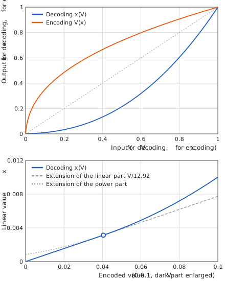
Before encoding, values that have become negative outside the color gamut are replaced by $0$ (because a power of a negative number is undefined). Both the decoded and the encoded results are confined to the range $0$ to $1$.

3. Conversion between RGB and XYZ

Let the linear RGB be the column vector $(R,G,B)^{\mathsf T}$, with the white point D65. The conversion matrices are derived from the chromaticities of the primaries and the white point as follows [7][8].

3-1. Derivation from the primaries and the white point

Let $(x_i,y_i)$ be the chromaticity of primary $i$ ($i=\mathrm{R},\mathrm{G},\mathrm{B}$), and define its direction vector

Let $P=[\mathbf{p}_{\mathrm R}\ \mathbf{p}_{\mathrm G}\ \mathbf{p}_{\mathrm B}]$ be the matrix having these vectors as columns, and let $\mathbf{W}$ be the vector of the same form for the chromaticity $(x_w,y_w)$ of the white point. The condition that white ($R=G=B=1$) is mapped to $\mathbf{W}$, namely $P\mathbf{S}=\mathbf{W}$, determines the strength coefficients of the primaries, $\mathbf{S}=P^{-1}\mathbf{W}$. The RGB → XYZ matrix is then

with which white has $Y=1$. The XYZ → RGB matrix is the exact inverse $M^{-1}$ of $M$.

3-2. sRGB

The chromaticities of the primaries are R$(0.64,\,0.33)$, G$(0.30,\,0.60)$, B$(0.15,\,0.06)$, and the white point is D65 with $(x,y)=(0.3127,\,0.3290)$ (IEC 61966-2-1 [2]). By §3-1, the values derived in double precision are, to seven digits,

The forward matrix given in the standard [2] to four decimal places (Eq. (7)) coincides with the derived values rounded to four digits.

The inverse matrix of the standard to four digits (Eq. (8)) is the rounded inverse of the rounded forward matrix, and therefore differs from the inverse of the derived matrix above in the fourth digit.

3-3. Display P3

The chromaticities of the primaries are R$(0.680,\,0.320)$, G$(0.265,\,0.690)$, B$(0.150,\,0.060)$, and the white point is D65 with $(0.3127,\,0.3290)$ (SMPTE EG 432-1 [3]; Apple's definition [4]). By §3-1 one obtains likewise

3-4. Exchanging color spaces

XYZ does not depend on the color space. Therefore, even when the input is sRGB and the output is Display P3, $u'$, $v'$ and $L^{*}$ take the same values on XYZ, and the same color keeps the same appearance while the wide gamut of P3 can be represented.

4. XYZ and CIELUV

4-1. Chromaticity $u',\,v'$

The chromaticity of the CIE 1976 UCS diagram is given by [6][7]

In terms of the $xy$ chromaticity,

For $X=Y=Z=0$ (black) the denominator vanishes, so the value of the D65 white, $(u'_n,\,v'_n)\approx(0.1978,\,0.4683)$, is used.

4-2. Lightness $L^{*}$

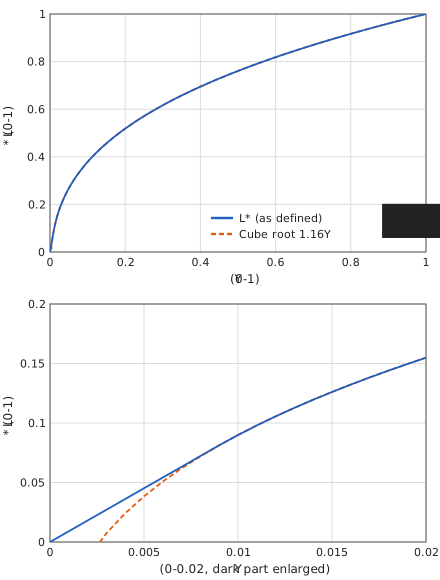
The CIE 1976 lightness (on the scale $0\le L^{*}\le 1$) is given by [6][7]

Here $9.033$ is $\frac{\kappa}{100}$ with $\kappa=\left(\frac{29}{3}\right)^{3}\approx 903.3$, and $0.008856$ corresponds to $\varepsilon=\left(\frac{6}{29}\right)^{3}$. This is the CIE definition $116\,f\!\left(\frac{Y}{Y_n}\right)-16$ divided by $100$, and the two expressions are continuous at the boundary $Y=\varepsilon$, where $L^{*}=0.0800$.

4-3. Inverse conversion

XYZ is obtained from the lightness after the transform, $L^{*}_{\mathrm{r}}$, and the chromaticity $(u',v')$ by

where $\frac{1}{9.033}\approx 0.11071$.

The boundary $L^{*}_{\mathrm{r}}=0.08$ corresponds to CIE $L^{*}=8$ ($=\frac{\kappa\varepsilon}{100}$). Eq. (15) is the definition of $u'$ and $v'$ in Eq. (11) solved for $X$ and $Z$; multiplication by $Y$ changes the brightness while the chromaticity stays unchanged.

5. Brighter

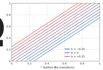
The value $b$ is added to the lightness before the transform, $L^{*}$, to give the lightness after the transform, $L^{*}_{\mathrm{b}}$.

A positive $b$ makes the whole image brighter and a negative $b$ makes it darker. The chromaticity is not changed.

6. Clearer

A logistic function normalized so that both ends coincide with $0$ and $1$ is applied to the lightness before the transform, $L^{*}_{\mathrm{b}}$, to give the lightness after the transform, $L^{*}_{\mathrm{c}}$.

Properties

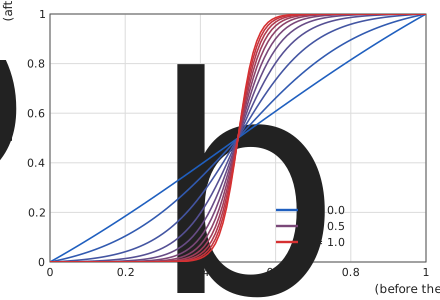
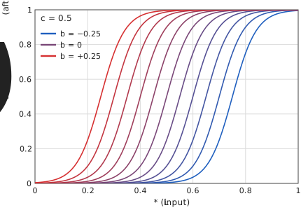
• End points and center: $L^{*}_{\mathrm{c}}=0$ at $L^{*}_{\mathrm{b}}=0$, $L^{*}_{\mathrm{c}}=1$ at $L^{*}_{\mathrm{b}}=1$, and $L^{*}_{\mathrm{c}}=0.5$ at $L^{*}_{\mathrm{b}}=0.5$. The curve is point-symmetric about the point $(0.5,\,0.5)$. The denominator $1-2y_0$ is the normalization that fits both ends to $0$ and $1$.
• Slope: The slope at $L^{*}_{\mathrm{b}}=0.5$ is
  $$\frac{dL^{*}_{\mathrm{c}}}{dL^{*}_{\mathrm{b}}}=\frac{t_0}{2\,(1-2y_0)} \tag{20}$$

  which is about $1.08$ for $c=0$, $5.5$ for $c=0.5$, and $10.5$ for $c=1$. The larger $c$ is, the steeper the curve is near the center: the dark side becomes darker and the light side becomes lighter, so that the difference between light and dark is emphasized.

• Inverse function: Put $y=L^{*}_{\mathrm{c}}\,(1-2y_0)+y_0$. Then

  $$L^{*}_{\mathrm{b}}=\frac{1}{2}\left(1-\frac{1}{t_0}\ln\!\left(\frac{1}{y}-1\right)\right) \tag{21}$$

• Even for $c=0$ the map is not the identity but a gentle S-shaped curve with $t_0=1$. The maximum deviation from the identity is $-0.0153$, at $L^{*}_{\mathrm{b}}=0.22$.
• Combination with Brighter: When $b$ is added, the center of the S-shaped curve (the point where $L^{*}_{\mathrm{c}}=0.5$) moves to $L^{*}=0.5-b$.
• Domain: For $b\ne 0$, $L^{*}_{\mathrm{b}}$ may extend outside $[0,1]$. In that case $L^{*}_{\mathrm{c}}$ may also extend outside $[0,1]$ (for example, for $c=0$ and $b=\pm 0.25$, $L^{*}_{\mathrm{c}}$ ranges from $-0.187$ to $1.187$). The larger $c$ is, the closer to $0$ or $1$ the outlying part falls asymptotically. Clipping to the displayable range is performed at the encoding stage of §2.

Origin

This S-shaped curve was inspired by the compression of the cone response. That the CIE lightness is expressed as the cube root of the intensity is known as a fit of Stevens' power law [9]. In contrast, the compression of the cone response is expressed by the following fractional function.

This is a function of the Naka–Rushton type [10], which has also been fitted to measurements of primate cones [11]. Similar compression is used in the compression stages of the color appearance models CIECAM02 [12] and CAM16 [13] (see [14] for an exposition). Plotted against the logarithm of the intensity, the fractional function draws the same S-shaped curve as the logistic function. The logistic function was adopted because the slope can be controlled by a single parameter $t_0$ and because the normalization that fits both ends to $0$ and $1$ is simple.

7. Brightness Reverse

From the lightness before the transform, $L^{*}_{\mathrm{c}}$, the lightness after the transform, $L^{*}_{\mathrm{r}}$, is defined by

When the reversal is not applied, $L^{*}_{\mathrm{r}}=L^{*}_{\mathrm{c}}$. The reversal is applied to $L^{*}_{\mathrm{c}}$. Since the S-shaped curve is point-symmetric about $(0.5,\,0.5)$, exchanging the order of the reversal and Clearer does not change the result when $b=0$. When $b\ne 0$, the result depends on the order.

8. Monochrome Mode

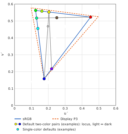
In Monochrome Mode, the chromaticity of the original pixel is discarded and replaced with a chromaticity obtained by mixing the $u'v'$ of a light color and a dark color by $L^{*}_{\mathrm{r}}$. The light color L and the dark color D are specified by sRGB values, and their chromaticities obtained by §4-1 are denoted $(u'_{\mathrm L},\,v'_{\mathrm L})$ and $(u'_{\mathrm D},\,v'_{\mathrm D})$.

• When L = D, the mode is one-color: the chromaticity is constant and only the brightness varies. When L ≠ D, the mode is two-color: the dark side approaches the tint of D and the light side that of L.
• The mixing is a linear interpolation on the $u'v'$ plane, not in $L^{*}$. The result lies on the line segment connecting the two points. Since the triangle of the color gamut is convex, the mixed chromaticity does not leave the gamut for $0\le L^{*}_{\mathrm{r}}\le 1$.
• When the light or dark color is black (XYZ all zero), the chromaticity of the D65 white is used, as in §4-1.

Clipping at the gamut boundary

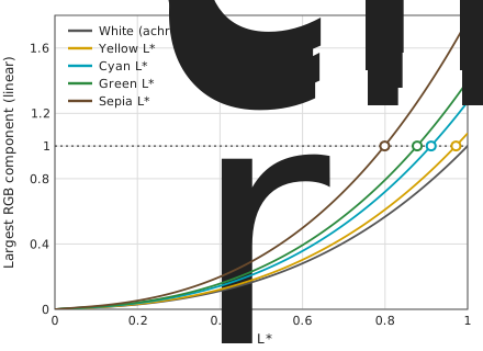
When $Y$ is increased with the chromaticity fixed, there is a point at which the linear RGB values exceed $1$ while the chromaticity is unchanged. The excess is clipped to $1$ by the encoding, and the tint moves toward white. For a color of chromaticity $(u',v')$, let $\mu$ be the largest linear RGB component per unit luminance ($Y=1$). Clipping begins at the luminance $Y=\frac{1}{\mu}$, that is,

This threshold depends on the color. Examples with sRGB linear RGB are given below.

The larger the largest component $\mu$ per unit luminance, the lower the threshold. For example, sepia has a small largest component, but when converted to unit luminance its $\mu$ is large, so its threshold is as low as $0.799$. In the two-color mode, the same threshold is determined for each mixed chromaticity.

9. Tilted Angle Correction (projection transform)

A sheet of paper photographed from an oblique direction is corrected to look as if viewed from directly above. The correction is represented by a single projective transformation $H$ that maps a point on the corrected screen to a point on the image.

9-1. Inverse of the perspective

The paper is assumed to be a plane whose center is crossed by the optical axis of the camera. The plane is tilted about a horizontal axis by a tilt angle $\theta$ ($0\le\theta<90^{\circ}$), with the upper part of the paper farther away. Taking the focal length as the unit of distance, let the distance from the camera to the center of the paper be $1$. A point $(x_p,\,y_p)$ on the paper lies at $(x_p,\ y_p\cos\theta,\ 1+y_p\sin\theta)$ in three dimensions, and its image coordinates $(\Xi,\,\Upsilon)$ (in units of the focal length) are

The normalized image coordinates $(u,v)$ (with the edges of the image at $\pm 1$) are related to these through the width $s_x$ and the height $s_y$ of the image and the focal length $f$ (in the same unit) by

Here $\xi$ and $\eta$ are the tangents of the half angles of view, and $\eta$ is the one in the vertical direction of the screen.

Let the normalized coordinates $(X,Y)$ of the corrected screen be proportional to the coordinates on the paper, $x_p=\xi X$ and $y_p=\eta Y$. Substituting these into Eq. (26) and solving for $u$ and $v$ gives the map from a point of the corrected screen to a point of the image.

This is the projective transformation, in homogeneous coordinates, given by the following $3\times 3$ matrix $Q^{-1}$.

Applying $Q^{-1}$ to $(X,Y,1)^{\mathsf T}$ gives $(u',\,v',\,w)^{\mathsf T}$, and $(u,v)=\left(\frac{u'}{w},\frac{v'}{w}\right)$. The case where the near side is the bottom side is shown. When the near side is the right, top, or left side, the matrix of the same form with the axes and signs exchanged is used.

The distance to the paper is not needed. Changing the distance only changes the overall scale of the corrected image.

The aspect ratio is preserved. The physical coordinates of the corrected screen, given the aspect ratio $\xi:\eta$ of the image, are $(\xi X,\ \eta Y)=(x_p,\ y_p)$. That is, the corrected image is the coordinates of the plane of the paper itself and is similar to it. Therefore ratios of lengths and angles are preserved, and a square sheet of paper is imaged as a square. This is the metric rectification of Hartley and Zisserman [15] (Section 2.7), applied to the case where the tilt is restricted to a horizontal axis.

9-2. Magnification that fills the margins

To keep the four corners of the corrected screen inside the image, the coordinates of the screen must be scaled by $\frac{1}{m}$. From the condition that the near corners $\left(\pm\frac{1}{m},\,-\frac{1}{m}\right)$ lie inside the image, $\dfrac{1/m}{1-\eta\sin\theta/m}\le 1$, the magnification is

($w>0$ is preserved as long as $\eta\sin\theta<1$). The value $m$ increases with $\theta$, and part of the edge of the image falls outside the screen.

9-3. The overall transformation

The transformation $H$ from a point on the screen (with coordinates normalized to the range $0$ to $1$) to a point on the image is the composition of the following maps.

Here $\mathrm{zoom}$ is the magnification, $\mathrm{pan}_x$ and $\mathrm{pan}_y$ are the shifts, and $h_x$ and $h_y$ are the ratios that make the image fill the screen (one of them is $1$). The transformation from the image to the screen is given by the inverse matrix of $H$, which is again a $3\times 3$ projective transformation.

References

[1] K. Asada, "Brighter and Bigger", README (appendix: mathematical expressions of the Brighter and Clearer theory), GitHub repository asada0/BrighterAndBigger, 2019, MIT License. https://github.com/asada0/BrighterAndBigger

[2] IEC 61966-2-1:1999, Multimedia systems and equipment — Colour measurement and management — Part 2-1: Colour management — Default RGB colour space — sRGB, International Electrotechnical Commission; and Amendment 1:2003 (published 23 January 2003).

[3] SMPTE EG 432-1:2010, Digital Source Processing — Color Processing for D-Cinema, Society of Motion Picture and Television Engineers, 10 November 2010. doi:10.5594/SMPTE.EG432-1.2010

[4] Apple Inc., "Display P3", ICC RGB Color Space Registry, International Color Consortium, version 1.0, 9 February 2022. https://registry.color.org/rgb-registry/displayp3 (accessed 22 October 2026). See also Apple Developer Documentation, CGColorSpace.displayP3, https://developer.apple.com/documentation/coregraphics/cgcolorspace/displayp3 (accessed 22 October 2026).

[5] T. Smith and J. Guild, "The C.I.E. colorimetric standards and their use", Transactions of the Optical Society, vol. 33, no. 3, pp. 73–134, 1931–32. doi:10.1088/1475-4878/33/3/301

[6] CIE 15:2004, Colorimetry, 3rd ed., Commission Internationale de l'Éclairage, 2004, ISBN 978-3-901906-33-6 (since superseded by CIE 015:2018).

[7] G. Wyszecki and W. S. Stiles, Color Science: Concepts and Methods, Quantitative Data and Formulae, 2nd ed., John Wiley & Sons, 1982, ISBN 978-0-471-02106-3.

[8] C. Poynton, Digital Video and HD: Algorithms and Interfaces, 2nd ed., Morgan Kaufmann, 2012, ISBN 978-0-12-391926-7.

[9] S. S. Stevens, "On the psychophysical law", Psychological Review, vol. 64, no. 3, pp. 153–181, 1957. doi:10.1037/h0046162

[10] K. I. Naka and W. A. H. Rushton, "S-potentials from colour units in the retina of fish (Cyprinidae)", The Journal of Physiology, vol. 185, no. 3, pp. 536–555, 1966. doi:10.1113/jphysiol.1966.sp008001

[11] J. M. Valeton and D. van Norren, "Light adaptation of primate cones: An analysis based on extracellular data", Vision Research, vol. 23, no. 12, pp. 1539–1547, 1983. doi:10.1016/0042-6989(83)90167-0

[12] CIE 159:2004, A Colour Appearance Model for Colour Management Systems: CIECAM02, Commission Internationale de l'Éclairage, 2004, ISBN 978-3-901906-29-9.

[13] C. Li, Z. Li, Z. Wang, Y. Xu, M. R. Luo, G. Cui, M. Melgosa, M. H. Brill, and M. Pointer, "Comprehensive color solutions: CAM16, CAT16, and CAM16-UCS", Color Research & Application, vol. 42, no. 6, pp. 703–718, 2017. doi:10.1002/col.22131

[14] M. D. Fairchild, Color Appearance Models, 3rd ed., John Wiley & Sons, 2013, ISBN 978-1-119-96703-3. doi:10.1002/9781118653128

[15] R. Hartley and A. Zisserman, Multiple View Geometry in Computer Vision, 2nd ed., Cambridge University Press, 2003, ISBN 978-0-521-54051-3. doi:10.1017/CBO9780511811685